9 Group 8
Managers: Bruna Cassoni, Daniela Locce, and Isabela Santos
9.1 The setup
p8_list  <-c("LREN3.SA","BPT","CRWD","PETR4.SA","VALE3.SA","HYPE3.SA","LCAM3.SA","MEGA3.SA","AURE3.SA","ITUB4.SA","TIMS3.SA","PETZ3.SA","ELET6.SA","JHSF3.SA","MOVI3.SA","BBDC4.SA","VIVA3.SA","BBSE3.SA","ARML3.SA","HAPV3.SA","TOTS3.SA","JBSS3.SA","VBBR3.SA","ETER3.SA","CIEL3.SA","GGBR4.SA")
p8_w     <- c("0.06", "0.04", "0.03", "0.08", "0.07", "0.06", "0.06", "0.05", "0.05", "0.05", "0.04", "0.04", "0.04", "0.04", "0.03", "0.03", "0.03", "0.03", "0.03", "0.03", "0.02", "0.04", "0.02", "0.01", "0.01", "0.01")
p8_exc   <- c("BRL","USD","USD","BRL","BRL","BRL","BRL","BRL","BRL","BRL","BRL","BRL","BRL","BRL","BRL","BRL","BRL","BRL","BRL","BRL","BRL","BRL","BRL","BRL","BRL","BRL")
p8_wlist <- cbind(p8_list, p8_w, p8_exc)
colnames(p8_wlist) <- c('ticker','weights','Currency')
#Download data Financial
p8 <- yf_get(tickers = p8_list, first_date = start, last_date = end,freq_data = "daily", thresh_bad_data = 0.5)
p8 <- p8[, c("ticker", "ref_date", "price_adjusted" ) ]
p8 <- merge(p8, p8_wlist , by = "ticker")
# Download data Exchange rate
getFX("BRL/USD",from=start , to = end)
exchanges <- as.data.frame(BRLUSD)
exchanges$ref_date <- as.Date(rownames(exchanges))
# Merge
p8 <- merge(p8, exchanges, by = "ref_date")
p8$BRL.USD[p8$Currency == "USD"] <- 1
# Adjusting currency
p8$price_adj <- p8$price_adjusted * p8$BRL.USD
# Calculating return
ret <- p8 %>%
       group_by(ticker) %>%
       tq_transmute(select = price_adj,
                    mutate_fun = periodReturn,
                    period = "daily",
                    col_rename = "ret")
p8 <- merge(p8, ret, by = c("ref_date", "ticker"))
# Data tabulation
p8$ret_product <- p8$ret * as.numeric(p8$weights)
# Creating a df of portfolios return
p8_ret  <- p8 %>%
            group_by(ref_date) %>%
            summarise_at(vars(ret_product),
                         list(p8_return = sum)) %>% as.data.frame()
#Calculating cumulative return per day
for(i in (1:nrow(p8_ret) ) ) {
p8_ret$p8_cum[i] <- Return.cumulative(p8_ret$p8_return[1:i])
}
#Calculating cumulative return total
p8_sharpe <- data.frame(matrix(NA, nrow = 1,ncol = 4))
colnames(p8_sharpe) <- c('p8_return', 'p8_sd', 'p8_rf' , 'p8_sharpe')
p8_sharpe$p8_return <- Return.cumulative(p8_ret$p8_return)
p8_sharpe$p8_sd <- sd(p8_ret$p8_return[2:nrow(p8_ret)])
p8_sharpe$p8_rf <- (1+0.03)^(nrow(p8_ret)/252) -1
p8_sharpe$p8_sharpe <- (p8_sharpe$p8_return - p8_sharpe$p8_rf)  / p8_sharpe$p8_sd
9.2 The portfolio
This is the portfolio of this group:
p8_wlist ticker weights Currency
[1,] "LREN3.SA" "0.06" "BRL"
[2,] "BPT" "0.04" "USD"
[3,] "CRWD" "0.03" "USD"
[4,] "PETR4.SA" "0.08" "BRL"
[5,] "VALE3.SA" "0.07" "BRL"
[6,] "HYPE3.SA" "0.06" "BRL"
[7,] "LCAM3.SA" "0.06" "BRL"
[8,] "MEGA3.SA" "0.05" "BRL"
[9,] "AURE3.SA" "0.05" "BRL"
[10,] "ITUB4.SA" "0.05" "BRL"
[11,] "TIMS3.SA" "0.04" "BRL"
[12,] "PETZ3.SA" "0.04" "BRL"
[13,] "ELET6.SA" "0.04" "BRL"
[14,] "JHSF3.SA" "0.04" "BRL"
[15,] "MOVI3.SA" "0.03" "BRL"
[16,] "BBDC4.SA" "0.03" "BRL"
[17,] "VIVA3.SA" "0.03" "BRL"
[18,] "BBSE3.SA" "0.03" "BRL"
[19,] "ARML3.SA" "0.03" "BRL"
[20,] "HAPV3.SA" "0.03" "BRL"
[21,] "TOTS3.SA" "0.02" "BRL"
[22,] "JBSS3.SA" "0.04" "BRL"
[23,] "VBBR3.SA" "0.02" "BRL"
[24,] "ETER3.SA" "0.01" "BRL"
[25,] "CIEL3.SA" "0.01" "BRL"
[26,] "GGBR4.SA" "0.01" "BRL" Checking the sum of weights. The sum of weights is:
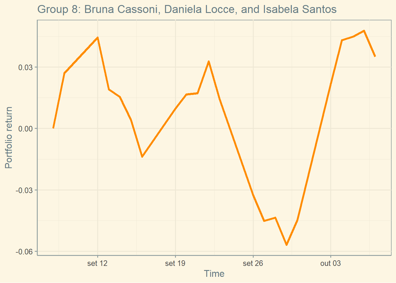
9.3 The performance
The current cumulative return of this Portfolio is 3.5 percent.
The current standard deviation of daily returns of this Portfolio is 2.37 percent.
The current Sharpe of this portfolio is 1.367.
ggplot(p8_ret, aes(x= ref_date, y= p8_cum) ) +  geom_line(color = "darkorange", size = 1.25) +
  labs(y = "Portfolio return",
       x = "Time",
       title = "Group 8: Bruna Cassoni, Daniela Locce, and Isabela Santos") + theme_solarized()