3  Group 2

Managers: Ana Paula Brandao, Manoela Brandi, Natalia Wakimoto

3.1 The setup

p2_list  <- c("COCA34.SA","IGTI3.SA","JBSS3.SA","MULT3.SA","PETR4.SA","RENT3.SA","T","XOM")
p2_w     <- c("0.23554", "0.00150", "0.15327", "0.01500", "0.13153", "0.01500", "0.01500", "0.43316")
p2_exc   <- c("BRL","BRL","BRL","BRL","BRL","BRL","USD","USD")
p2_wlist <- cbind(p2_list, p2_w, p2_exc)
colnames(p2_wlist) <- c('ticker','weights','Currency')
#Download data Financial
p2 <- yf_get(tickers = p2_list, first_date = start, last_date = end,freq_data = "daily", thresh_bad_data = 0.5)
p2 <- p2[, c("ticker", "ref_date", "price_adjusted" ) ]
p2 <- merge(p2, p2_wlist , by = "ticker")
# Download data Exchange rate
getFX("BRL/USD",from=start , to = end) 
exchanges <- as.data.frame(BRLUSD)
exchanges$ref_date <- as.Date(rownames(exchanges))
# Merge
p2 <- merge(p2, exchanges, by = "ref_date")
p2$BRL.USD[p2$Currency == "USD"] <- 1
# Adjusting currency
p2$price_adj <- p2$price_adjusted * p2$BRL.USD
# Calculating return
ret <- p2 %>%
       group_by(ticker) %>%
       tq_transmute(select = price_adj,
                    mutate_fun = periodReturn,
                    period = "daily",
                    col_rename = "ret")
p2 <- merge(p2, ret, by = c("ref_date", "ticker"))
# Data tabulation
p2$ret_product <- p2$ret * as.numeric(p2$weights)
# Creating a df of portfolios return
p2_ret  <- p2 %>%                      
            group_by(ref_date) %>%
            summarise_at(vars(ret_product),
                         list(p2_return = sum)) %>% as.data.frame()
#Calculating cumulative return per day
for(i in (1:nrow(p2_ret) ) ) {
p2_ret$p2_cum[i] <- Return.cumulative(p2_ret$p2_return[1:i])
}
#Calculating cumulative return total
p2_sharpe <- data.frame(matrix(NA, nrow = 1,ncol = 4))
colnames(p2_sharpe) <- c('p2_return', 'p2_sd', 'p2_rf' , 'p2_sharpe')
p2_sharpe$p2_return <- Return.cumulative(p2_ret$p2_return)
p2_sharpe$p2_sd <- sd(p2_ret$p2_return[2:nrow(p2_ret)])
p2_sharpe$p2_rf <- (1+0.03)^(nrow(p2_ret)/252) -1
p2_sharpe$p2_sharpe <- (p2_sharpe$p2_return - p2_sharpe$p2_rf)  / p2_sharpe$p2_sd

3.2 The portfolio

This is the portfolio of this group:

p2_wlist

     ticker      weights   Currency
[1,] "COCA34.SA" "0.23554" "BRL"   
[2,] "IGTI3.SA"  "0.00150" "BRL"   
[3,] "JBSS3.SA"  "0.15327" "BRL"   
[4,] "MULT3.SA"  "0.01500" "BRL"   
[5,] "PETR4.SA"  "0.13153" "BRL"   
[6,] "RENT3.SA"  "0.01500" "BRL"   
[7,] "T"         "0.01500" "USD"   
[8,] "XOM"       "0.43316" "USD"   

Checking the sum of weights. The sum of weights is:

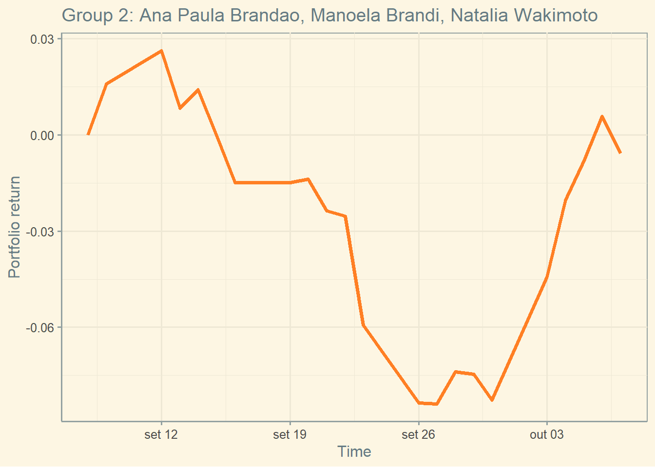
3.3 The performance

The current cumulative return of this Portfolio is -0.58 percent.

The current standard deviation of daily returns of this Portfolio is 1.75 percent.

The current Sharpe of this portfolio is -0.4794.

ggplot(p2_ret, aes(x= ref_date, y= p2_cum) ) +  geom_line(color = "chocolate1", size = 1.25) +
  labs(y = "Portfolio return", 
       x = "Time",
       title = "Group 2: Ana Paula Brandao, Manoela Brandi, Natalia Wakimoto") + theme_solarized()