5 Group 4
Managers: Gabriela Falcone, Gabriela Ricci, and JoC#o Gomes
5.1 The setup
p4_list  <- c("META","AMZN","DIS","GOOG","BLK","BRK","BFH","PAM","BABA","MU","DIBS","VST","JPM","VZ","BTI","WFC","BK","HPQ","BLAU3.SA","BBAS3.SA","ENBR3.SA","EZTC3.SA","MOVI3.SA","PNVL3.SA","VALE3.SA","EGIE3.SA","BBSE3.SA","PETR4.SA","AGRO3.SA","TUPY3.SA","ELET6.SA","ENBR3.SA","UNIP6.SA","LEVE3.SA","GRND3.SA")
p4_w     <- c("0.040","0.030","0.010","0.015","0.010","0.005","0.050","0.035","0.020","0.020","0.020","0.050","0.015","0.015","0.020","0.015","0.020","0.030","0.060","0.065","0.025","0.055","0.020","0.005","0.045","0.060","0.030","0.040","0.015","0.035","0.040","0.035","0.010","0.025","0.015")
p4_exc   <- c("USD","USD","USD","USD","USD","USD","USD","USD","USD","USD","USD","USD","USD","USD","USD","USD","USD","USD","BRL","BRL","BRL","BRL","BRL","BRL","BRL","BRL","BRL","BRL","BRL","BRL","BRL","BRL","BRL","BRL","BRL")

p4_wlist <- cbind(p4_list, p4_w, p4_exc)
colnames(p4_wlist) <- c('ticker','weights','Currency')
#Download data Financial
p4 <- yf_get(tickers = p4_list, first_date = start, last_date = end,freq_data = "daily", thresh_bad_data = 0.5)
p4 <- p4[, c("ticker", "ref_date", "price_adjusted" ) ]
p4 <- merge(p4, p4_wlist , by = "ticker")
# Download data Exchange rate
getFX("BRL/USD",from=start , to = end)
exchanges <- as.data.frame(BRLUSD)
exchanges$ref_date <- as.Date(rownames(exchanges))
# Merge
p4 <- merge(p4, exchanges, by = "ref_date")
p4$BRL.USD[p4$Currency == "USD"] <- 1
# Adjusting currency
p4$price_adj <- p4$price_adjusted * p4$BRL.USD
# Calculating return
ret <- p4 %>%
       group_by(ticker) %>%
       tq_transmute(select = price_adj,
                    mutate_fun = periodReturn,
                    period = "daily",
                    col_rename = "ret")
p4 <- merge(p4, ret, by = c("ref_date", "ticker"))
# Data tabulation
p4$ret_product <- p4$ret * as.numeric(p4$weights)
# Creating a df of portfolios return
p4_ret  <- p4 %>%
            group_by(ref_date) %>%
            summarise_at(vars(ret_product),
                         list(p4_return = sum)) %>% as.data.frame()
#Calculating cumulative return per day
for(i in (1:nrow(p4_ret) ) ) {
p4_ret$p4_cum[i] <- Return.cumulative(p4_ret$p4_return[1:i])
}
#Calculating cumulative return total
p4_sharpe <- data.frame(matrix(NA, nrow = 1,ncol = 4))
colnames(p4_sharpe) <- c('p4_return', 'p4_sd', 'p4_rf' , 'p4_sharpe')
p4_sharpe$p4_return <- Return.cumulative(p4_ret$p4_return)
p4_sharpe$p4_sd <- sd(p4_ret$p4_return[2:nrow(p4_ret)])
p4_sharpe$p4_rf <- (1+0.03)^(nrow(p4_ret)/252) -1
p4_sharpe$p4_sharpe <- (p4_sharpe$p4_return - p4_sharpe$p4_rf)  / p4_sharpe$p4_sd
5.2 The portfolio
This is the portfolio of this group:
p4_wlist ticker weights Currency
[1,] "META" "0.040" "USD"
[2,] "AMZN" "0.030" "USD"
[3,] "DIS" "0.010" "USD"
[4,] "GOOG" "0.015" "USD"
[5,] "BLK" "0.010" "USD"
[6,] "BRK" "0.005" "USD"
[7,] "BFH" "0.050" "USD"
[8,] "PAM" "0.035" "USD"
[9,] "BABA" "0.020" "USD"
[10,] "MU" "0.020" "USD"
[11,] "DIBS" "0.020" "USD"
[12,] "VST" "0.050" "USD"
[13,] "JPM" "0.015" "USD"
[14,] "VZ" "0.015" "USD"
[15,] "BTI" "0.020" "USD"
[16,] "WFC" "0.015" "USD"
[17,] "BK" "0.020" "USD"
[18,] "HPQ" "0.030" "USD"
[19,] "BLAU3.SA" "0.060" "BRL"
[20,] "BBAS3.SA" "0.065" "BRL"
[21,] "ENBR3.SA" "0.025" "BRL"
[22,] "EZTC3.SA" "0.055" "BRL"
[23,] "MOVI3.SA" "0.020" "BRL"
[24,] "PNVL3.SA" "0.005" "BRL"
[25,] "VALE3.SA" "0.045" "BRL"
[26,] "EGIE3.SA" "0.060" "BRL"
[27,] "BBSE3.SA" "0.030" "BRL"
[28,] "PETR4.SA" "0.040" "BRL"
[29,] "AGRO3.SA" "0.015" "BRL"
[30,] "TUPY3.SA" "0.035" "BRL"
[31,] "ELET6.SA" "0.040" "BRL"
[32,] "ENBR3.SA" "0.035" "BRL"
[33,] "UNIP6.SA" "0.010" "BRL"
[34,] "LEVE3.SA" "0.025" "BRL"
[35,] "GRND3.SA" "0.015" "BRL" Checking the sum of weights. The sum of weights is:
5.3 The performance
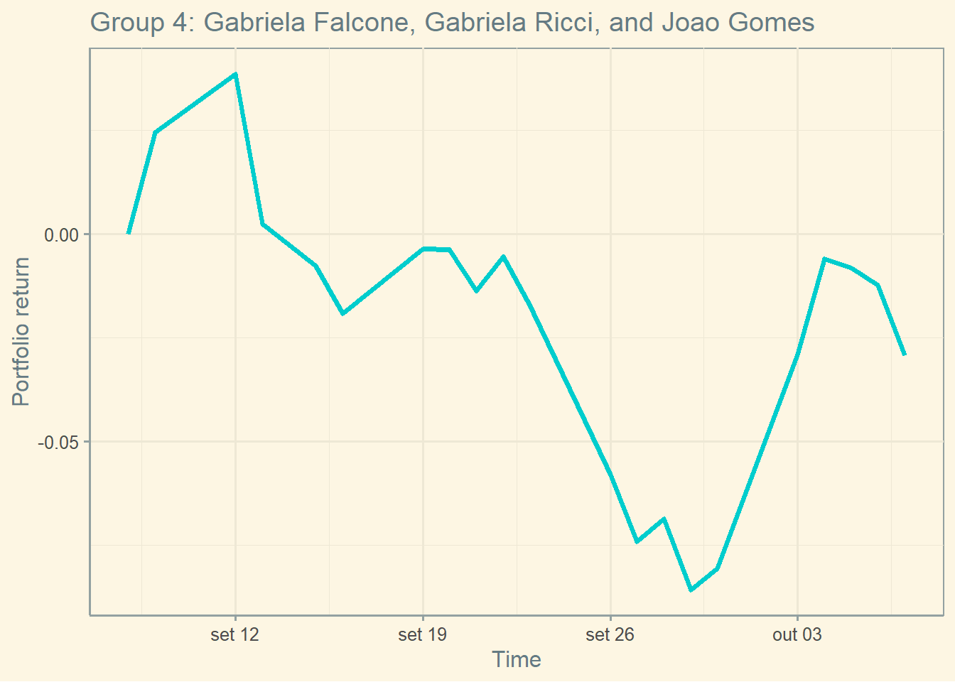
The current cumulative return of this Portfolio is -2.93 percent.
The current standard deviation of daily returns of this Portfolio is 2.14 percent.
The current Sharpe of this portfolio is -1.4905.
ggplot(p4_ret, aes(x= ref_date, y= p4_cum) ) +  geom_line(color = "cyan3", size = 1.25) +
  labs(y = "Portfolio return",
       x = "Time",
       title = "Group 4: Gabriela Falcone, Gabriela Ricci, and Joao Gomes") + theme_solarized()