6 Group 5
Managers: Isabella Piotto, Luiza Kneese, and Raquel Sanches
6.1 The setup
p5_list  <- c("WEC","MCK","COP","MPC","CVX","HRB","VLO","PXD","EOG","ED","CPB","OSI","AZO","WRB","ARX.TO","BTE.TO","CTRA","PNE.TO","TOU.TO","BANF","GBRG","AGBA","VENA","DWIN","VEDL","BPT","ARLP","PBT","XOM","MDP.TO","GIS")
p5_w     <- c("0.010","0.035","0.025","0.025","0.025","0.025","0.025","0.025","0.025","0.025","0.025","0.025","0.025","0.025","0.050","0.050","0.025","0.050","0.050","0.050","0.030","0.030","0.030","0.030","0.050","0.060","0.040","0.035","0.025","0.025","0.025")
p5_exc   <- c("USD","USD","USD","USD","USD","USD","USD","USD","USD","USD","USD","USD","USD","USD","CAD","CAD","USD","CAD","CAD","USD","USD","USD","USD","USD","USD","USD","USD","USD","USD","CAD","USD"  )
p5_wlist <- cbind(p5_list, p5_w, p5_exc)
colnames(p5_wlist) <- c('ticker','weights','Currency')
#Download data Financial
p5 <- yf_get(tickers = p5_list, first_date = start, last_date = end,freq_data = "daily", thresh_bad_data = 0.5)
p5 <- p5[, c("ticker", "ref_date", "price_adjusted" ) ]
p5 <- merge(p5, p5_wlist , by = "ticker")
# Download data Exchange rate
getFX("CAD/USD",from=start , to = end)
exchanges <- as.data.frame(CADUSD)
exchanges$ref_date <- as.Date(rownames(exchanges))
# Merge
p5 <- merge(p5, exchanges, by = "ref_date")
p5$CAD.USD[p5$Currency == "USD"] <- 1
# Adjusting currency
p5$price_adj <- p5$price_adjusted * p5$CAD.USD
# Calculating return
ret <- p5 %>%
       group_by(ticker) %>%
       tq_transmute(select = price_adj,
                    mutate_fun = periodReturn,
                    period = "daily",
                    col_rename = "ret")
p5 <- merge(p5, ret, by = c("ref_date", "ticker"))
# Data tabulation
p5$ret_product <- p5$ret * as.numeric(p5$weights)
# Creating a df of portfolios return
p5_ret  <- p5 %>%
            group_by(ref_date) %>%
            summarise_at(vars(ret_product),
                         list(p5_return = sum)) %>% as.data.frame()
#Calculating cumulative return per day
for(i in (1:nrow(p5_ret) ) ) {
p5_ret$p5_cum[i] <- Return.cumulative(p5_ret$p5_return[1:i])
}
#Calculating cumulative return total
p5_sharpe <- data.frame(matrix(NA, nrow = 1,ncol = 4))
colnames(p5_sharpe) <- c('p5_return', 'p5_sd', 'p5_rf' , 'p5_sharpe')
p5_sharpe$p5_return <- Return.cumulative(p5_ret$p5_return)
p5_sharpe$p5_sd <- sd(p5_ret$p5_return[2:nrow(p5_ret)])
p5_sharpe$p5_rf <- (1+0.03)^(nrow(p5_ret)/252) -1
p5_sharpe$p5_sharpe <- (p5_sharpe$p5_return - p5_sharpe$p5_rf)  / p5_sharpe$p5_sd
6.2 The portfolio
This is the portfolio of this group:
p5_wlist ticker weights Currency
[1,] "WEC" "0.010" "USD"
[2,] "MCK" "0.035" "USD"
[3,] "COP" "0.025" "USD"
[4,] "MPC" "0.025" "USD"
[5,] "CVX" "0.025" "USD"
[6,] "HRB" "0.025" "USD"
[7,] "VLO" "0.025" "USD"
[8,] "PXD" "0.025" "USD"
[9,] "EOG" "0.025" "USD"
[10,] "ED" "0.025" "USD"
[11,] "CPB" "0.025" "USD"
[12,] "OSI" "0.025" "USD"
[13,] "AZO" "0.025" "USD"
[14,] "WRB" "0.025" "USD"
[15,] "ARX.TO" "0.050" "CAD"
[16,] "BTE.TO" "0.050" "CAD"
[17,] "CTRA" "0.025" "USD"
[18,] "PNE.TO" "0.050" "CAD"
[19,] "TOU.TO" "0.050" "CAD"
[20,] "BANF" "0.050" "USD"
[21,] "GBRG" "0.030" "USD"
[22,] "AGBA" "0.030" "USD"
[23,] "VENA" "0.030" "USD"
[24,] "DWIN" "0.030" "USD"
[25,] "VEDL" "0.050" "USD"
[26,] "BPT" "0.060" "USD"
[27,] "ARLP" "0.040" "USD"
[28,] "PBT" "0.035" "USD"
[29,] "XOM" "0.025" "USD"
[30,] "MDP.TO" "0.025" "CAD"
[31,] "GIS" "0.025" "USD" Checking the sum of weights. The sum of weights is:
6.3 The performance
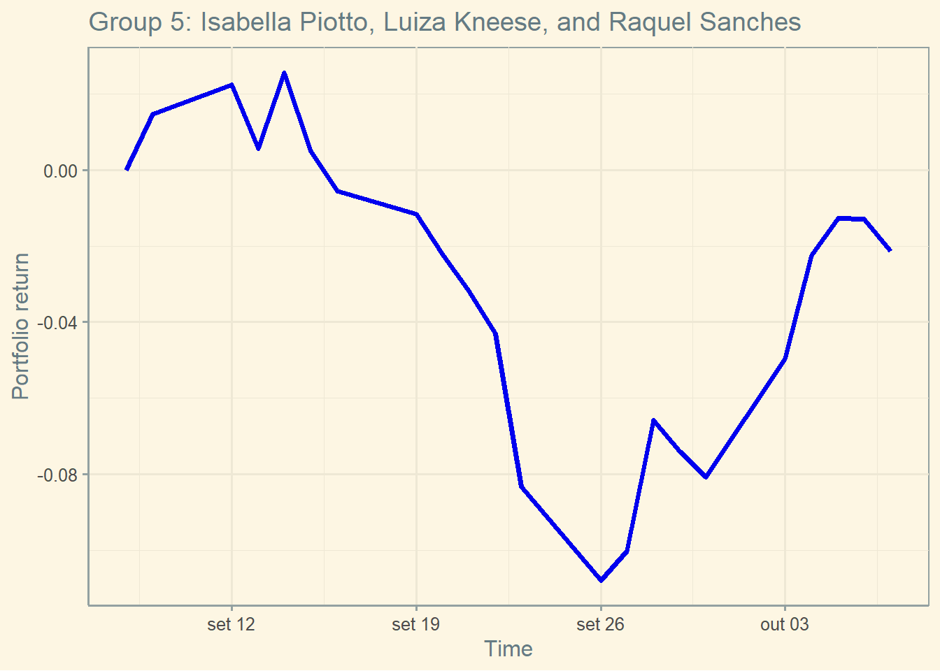
The current cumulative return of this Portfolio is -2.14 percent.
The current standard deviation of daily returns of this Portfolio is 2.01 percent.
The current Sharpe of this portfolio is -1.1929.
ggplot(p5_ret, aes(x= ref_date, y= p5_cum) ) +  geom_line(color = "blue2", size = 1.25) +
  labs(y = "Portfolio return",
       x = "Time",
       title = "Group 5: Isabella Piotto, Luiza Kneese, and Raquel Sanches") + theme_solarized()