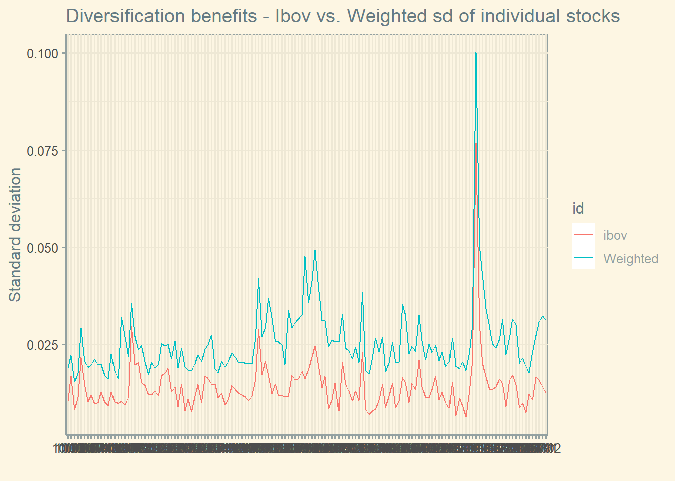
In this graph, we observe the benefits of diversification. The pink line computes the standard deviation of Ibov from 2010 to 2022, while the light green line computes the average of the standard deviation of the individual stocks that compose Ibov weighted by monthly volume. We can see that the portfolio has a lower standard deviation than the weighted average.
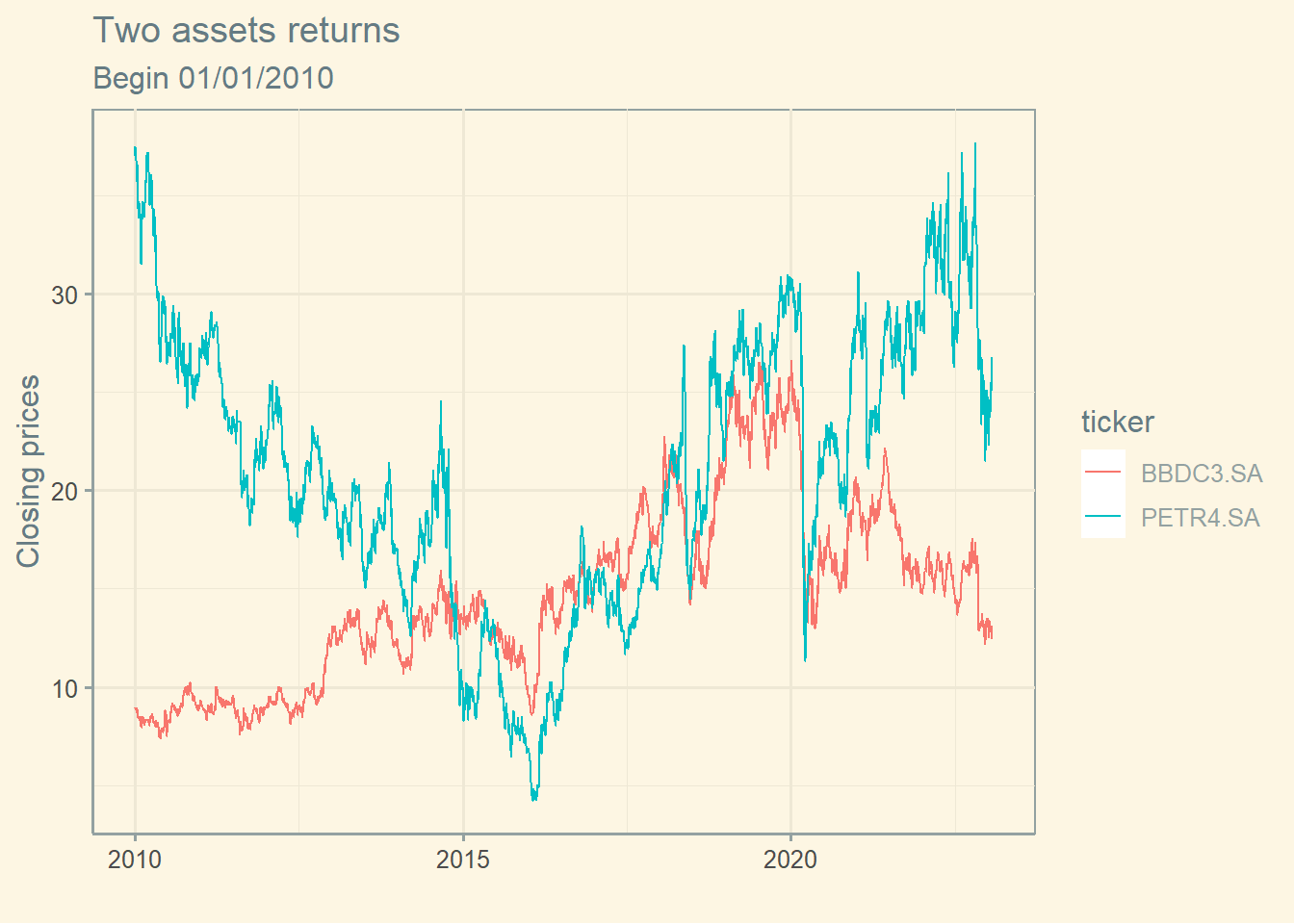
Note below that often when the price of a asset drops, the price of the other rises.
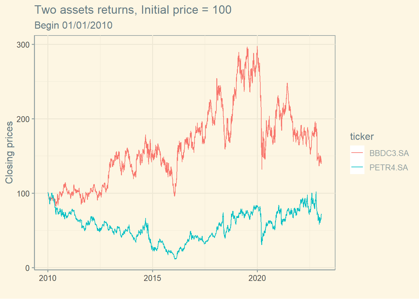
Let’s see the same graph using prices in day 1 = $100.
4.1.2 Correlation
Finally, let’s compute the correlation between the returns of these assets.
## [1] 0.5443201
The correlation is 0.544
4.1.3 Two-asset portfolio return
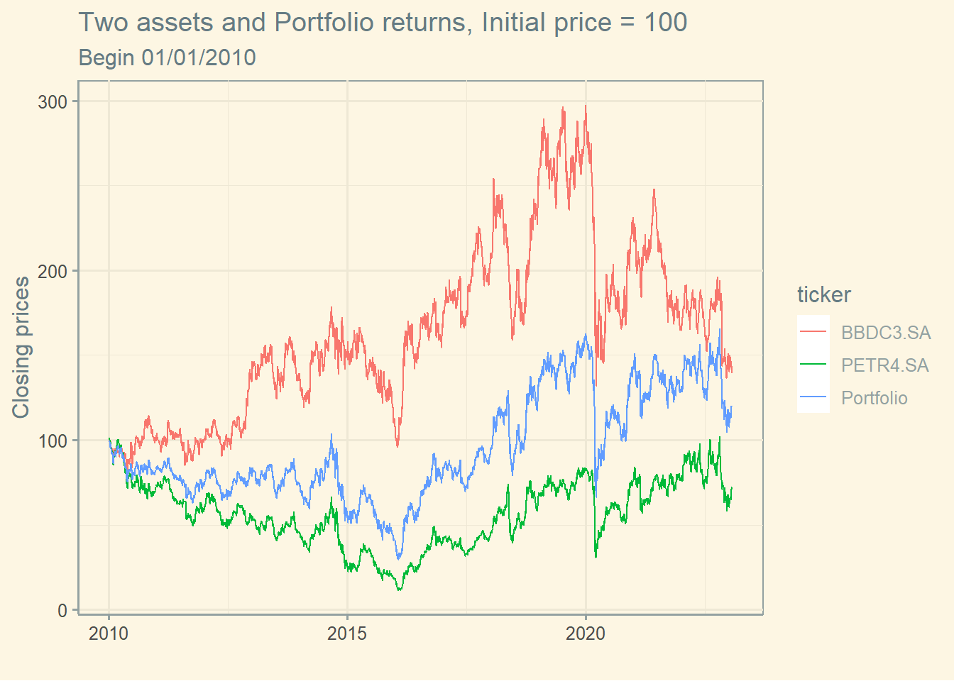
Now, let’s compute the average return of a portfolio with 40% invested in asset 1 and the remaining 60% invested in asset 2.
# Defining weights and calculating portfolio return (daily)w <-c(0.40, 0.60)# Creating a df with stocks and weightsw_tbl <-tibble(ticker = stocks,w = w)# Including the weights in the df prices (which contains the prices)prices <-left_join(data ,w_tbl, by ='ticker')# calculating the product of return times the portfolio weights for all days (this is necessary to calculate average return)prices$w_ret <- prices$ret_closing_prices * prices$w# Creating a dataframe with portfolio returns port_ret <- prices %>%group_by(ref_date) %>%summarise(port_ret =sum(w_ret))# Creating prices from the vector of returnsport_ret$price_close2 <-cumprod(1+port_ret$port_ret) *100# Graph with all returnsport_ret$ticker <-'Portfolio'ggplot(stock1, aes(ref_date , price_close2, color = ticker))+geom_line() +geom_line(data=stock2) +geom_line(data=port_ret) +labs(x ="",y='Closing prices', title="Two assets and Portfolio returns, Initial price = 100", subtitle ="Begin 01/01/2010") +theme_solarized()
Obs: The return of the portfolio is the weighted average of the assets’ returns.
## [1] 0.03216604
## [1] 0.03330732
The average return of asset 1 and asset 2 are, respectively, 0.032 and 0.033.
## [1] 0.03285081
The average return of the portfolio is 0.033. ___
We can compute the average return of the portfolio “by hand”:
[1] 0.03285081
The average return of the portfolio, computed by hand, is 0.033.
Notice below that the difference between the two methods of calculation is zero, as it should be!
[1] 0
4.2 Portfolio risk
4.2.1 Two-asset portfolio risk
However, the standard deviation of the portfolio returns is not the weighted average of the assets’ standard deviation. Remember the equation below:
These are the estimates from the previous example:
The standard deviation of asset 1 is 2.116.
The standard deviation of asset 2 is 2.932.
The standard deviation of the portfolio is 2.331.
The weighted average of the assets’ standard deviation is 2.606.
The decrease in the standard deviation due to diversification is -0.275.
4.2.2 Multi-assets portfolio risk
While the expected return of a three-asset portfolio is the weighted average of expected returns, the variance of the portfolio is measured using the equation below:
When you have enough stocks (with equal weights), you can compute the variance as follows:
\[Var=\frac{1}{N} \times average\;variance + (1-\frac{1}{N}) \times average \; covariance\]
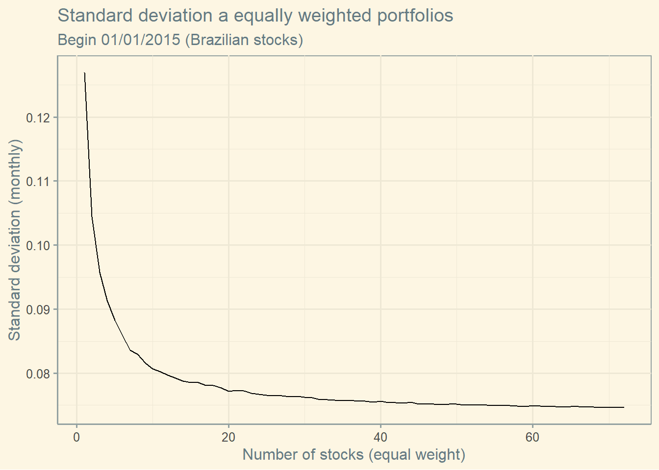
So, now, let’s compute the variance of multi-assets portfolios, equally weighted using real data from the Brazilian market.
start <-'2015-01-01'end <-'2022-01-01'# Finding the tickersdata_temp <-yf_collection_get("IBOV", first_date = start,last_date = end,freq_data ="monthly")tickers<-unique(data_temp$ticker)df <- data_temp %>%select(ref_date) %>%distinct()# Now collecting datafor (i in1:length(tickers)) {data <-yf_get(tickers[[i]], first_date = start,last_date = end,freq_data ="monthly")data <- data[complete.cases(data),] data <- data %>%select(ref_date, ret_closing_prices)colnames(data) <-c("ref_date", tickers[[i]] )df <-merge(df,data,by="ref_date")}# Setup to randomly combine "j" stocks and compute the standard deviation of this combinationfinal <-data.frame(matrix(NA,nrow =1000, ncol =length(tickers)))df$ref_date <-NULLfor (j in1:length(tickers) ) {for (i in1:2000 ) {df_r <-as.data.frame(df[, sample( ncol(df) , j )])cov <-cov(df_r)# Var meanvar <-as.data.frame(diag(cov))var_mean <-mean(var$`diag(cov)`)#Covariance meanif (j ==1) { covar_mean <- var_mean } else { covar <- covdiag(covar)=NA covar[upper.tri(covar)] <-NA covar<-c(covar) covar_mean<-mean(covar,na.rm=TRUE) }# Port Sd.var_p <- ( (1/ j * var_mean ) + (1- (1/j ) ) * covar_mean ) ^0.5final[i,j] <- var_p}}# Computing the average of the "i" portfolios with "j" stocks sd <-as.data.frame(colMeans(final))sd$N <-seq_along(sd[,1])ggplot(sd, aes(y=`colMeans(final)` , x = N)) +geom_line() +labs(x ="Number of stocks (equal weight)",y='Standard deviation (monthly)', title="Standard deviation a equally weighted portfolios", subtitle ="Begin 01/01/2015 (Brazilian stocks)") +theme_solarized()
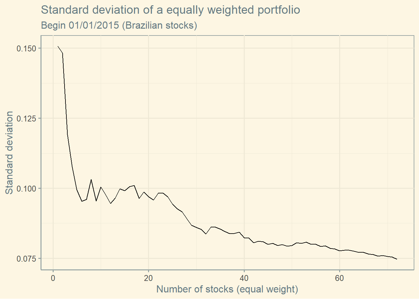
You see, the previous graph contains the average of all possible combinations using N stocks. The inclusion of the next stock is defined by volume. If you don’t take the average of all possible combinations, you get the next graph. Clearly, the drop in risk is not so smooth.
4.3 Correlation extended
See what happens with the portfolio risk when we change the combination of weights of each asset.
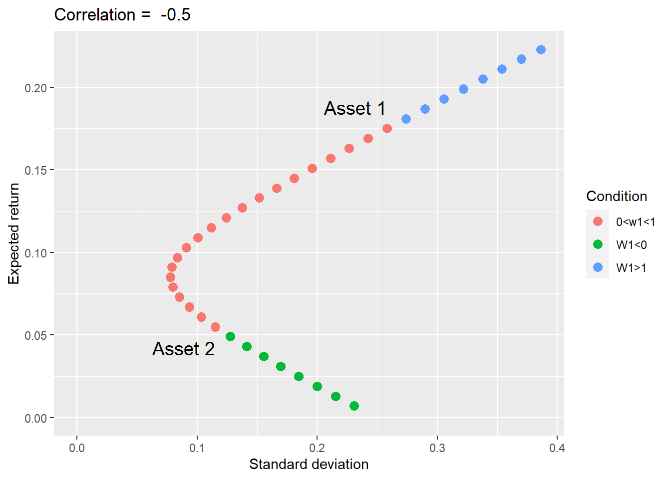
The graph below contains the set of feasible portfolios (i.e., investment possibilities) containing a combination of two assets. For this example, I am fabricating the data as below. The graph below suggests there is one combination of weights that minimizes the standard deviation of the portfolio.
Notice that this graph expands the weights to below zero and above one. These weights’ values occur when you can sell one asset to buy the other. The portfolios in which you are selling either one of the assets are represented in both outer parts of the curve.
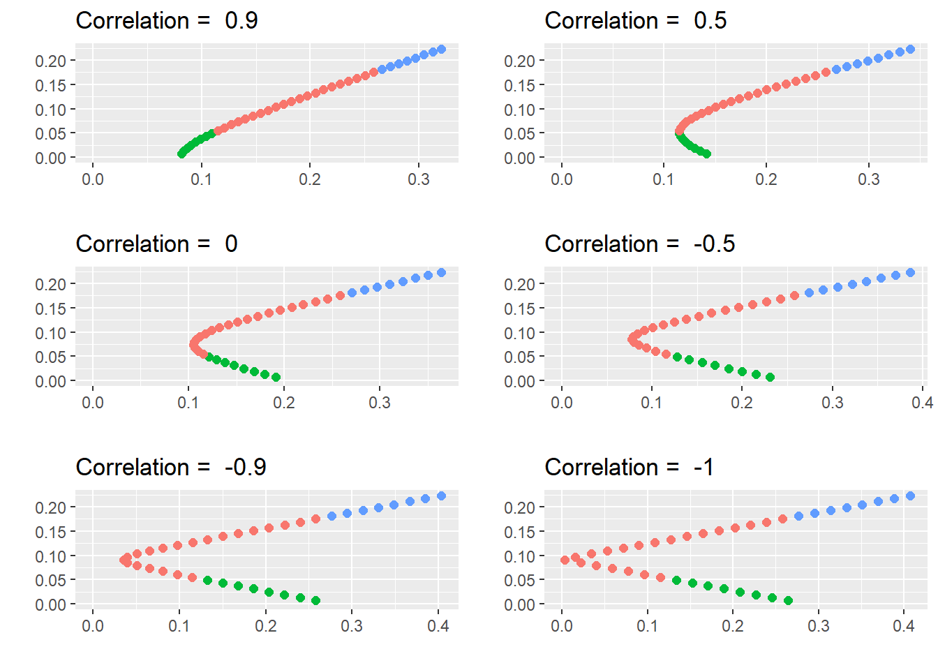
Let’s now change the correlation coefficient between these assets to see what happens.
That is, the shape of the investment possibilities is very sensitive to the correlation coefficient, especially when the correlation is negative.
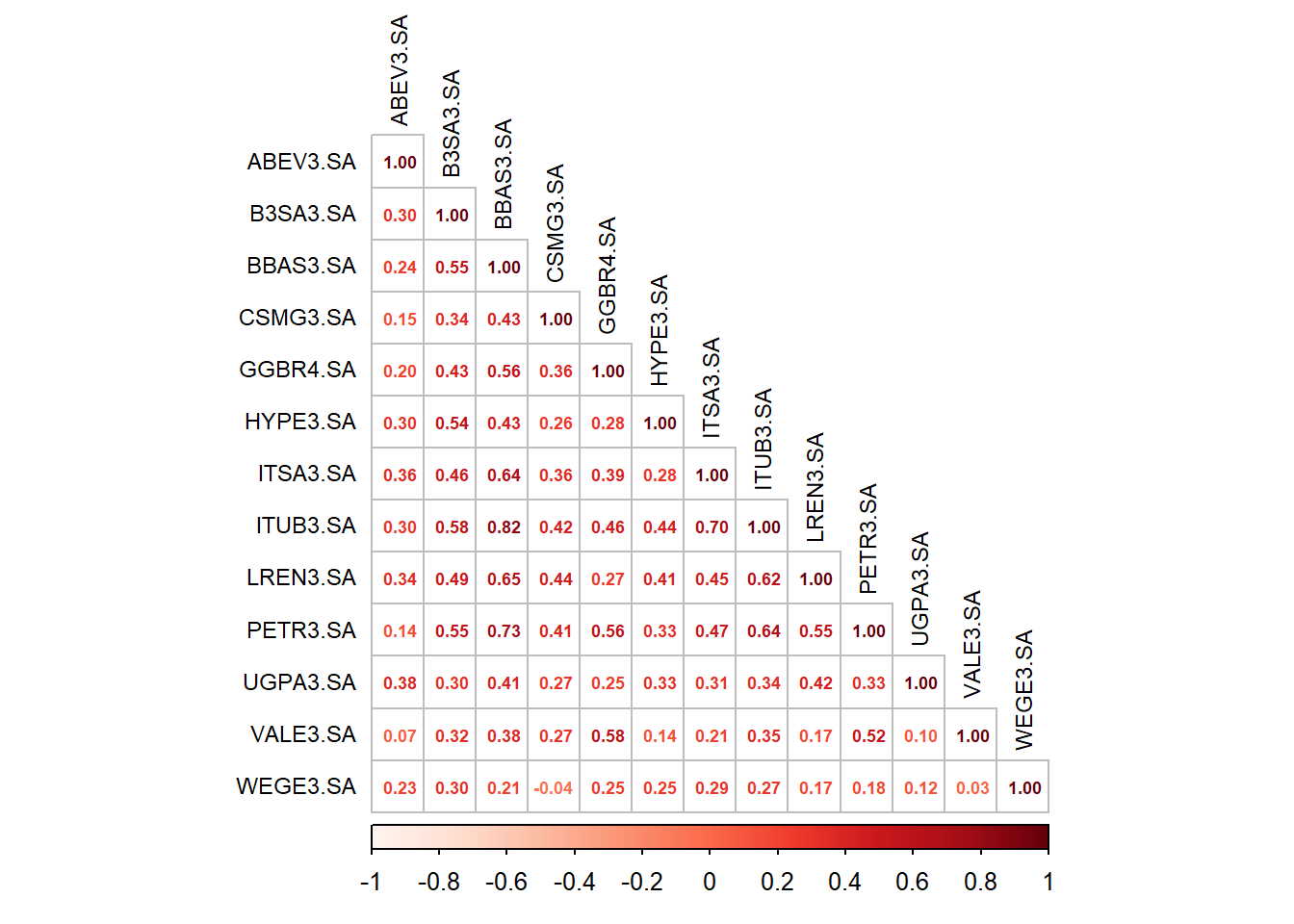
4.3.2 Correlation matrix Brazil
Here are some correlations between selected Brazilian stocks using montly data since 2010. As you can see, correlations are all positive and only a few are close to zero.
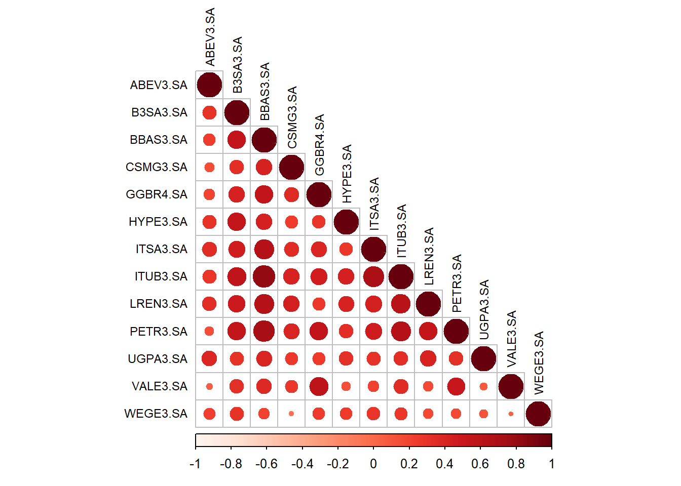
Let’s see the correlations using circles to improve the visuals.
corrplot(cor,method ='circle', type ='lower' , tl.col ="black", order ='alphabet', tl.cex =0.75, col =COL1('Reds') )
4.4 Efficient frontier
4.4.1 Minimum variance portfolio
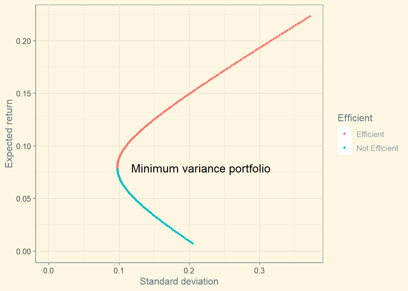
Before we create a graph of the efficient frontier using real data, let’s go back to fabricated data to visualize the efficient frontier and the minimum variance portfolio.
Below, you can see clearly that the portfolio closest to the y-axis is the one with minimum variance.This portfolio is important because it is at the beginning of the efficient frontier. All portfolios below are not optimal (because there is one portfolio in the frontier with the same level of risk but higher return).
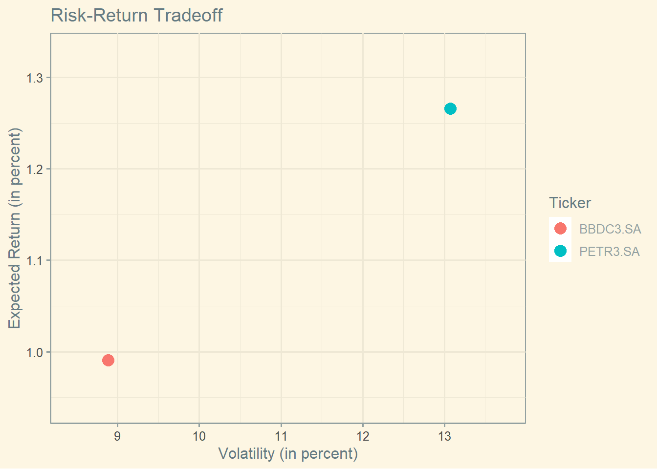
4.4.2 The historical returns and standard deviation of two assets
Let’s now move to an efficient frontier example using real data from Brazil. First, let’s download and compute the average return and the standard deviation of returns for two Brazilian stocks.
This is the representation in a graph, when return is on the y-asis and the standard deviation is on the x-axis.
4.4.4 The frontier using two assets
It is not as beautiful as the graph using fabricated data because the real correlation between these assets are not low. But notice that the shape is the same as before. Also notice that we can see the minimum variance portfolio as well.
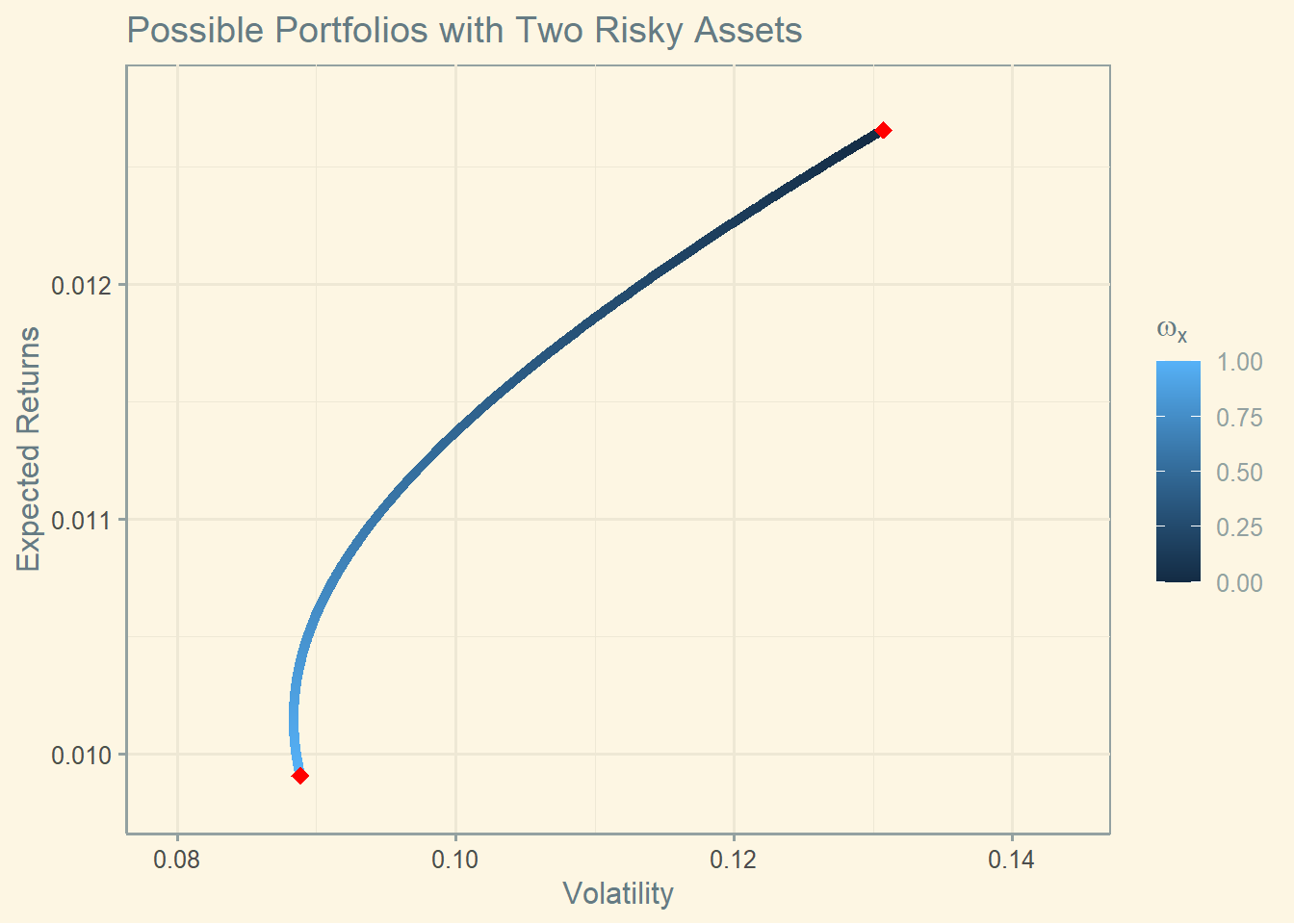
library(data.table)cov_12 <-cov(asset1$ret_adjusted_prices, asset2$ret_adjusted_prices)corr_12 <-cor(asset1$ret_adjusted_prices, asset2$ret_adjusted_prices)weights <-seq(from =0, to =1, length.out =1000)two_assets <-data.table(w1 = weights ,w2 =1- weights)# calculate the expected returns and standard deviations for the 1000 possible portfoliostwo_assets[, ':=' (er_p = w1 * er_1 + w2 * er_2,sd_p =sqrt(w1^2* sd_1^2+w2^2* sd_2^2+2* w1 * w2 * cov_12))]ggplot() +geom_point(data = two_assets, aes(x = sd_p, y = er_p, color = w1)) +geom_point(data =data.table(sd =c(sd_1, sd_2), mean =c(er_1, er_2)),aes(x = sd, y = mean), color ="red", size =3, shape =18) +theme_bw() +ggtitle("Possible Portfolios with Two Risky Assets") +xlab("Volatility") +ylab("Expected Returns") +scale_y_continuous( limits =c(min(two_assets$er_p)*0.99, max(two_assets$er_p)*1.01)) +scale_x_continuous( limits =c(min(two_assets$sd_p)*0.9, max(two_assets$sd_p)*1.1)) +scale_color_continuous(name =expression(omega[x]))+theme_solarized()
The correlation between these assets is 0.595, which explains the shape of the curve. Keep in mind that it is hard to find stocks with low correlations. You might find low correlation in more international markets. Not so much in Brazil. (Code inspired in: https://github.com/DavZim/Efficient_Frontier).
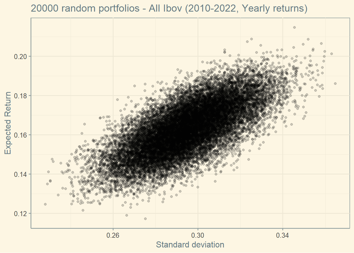
4.4.5 The frontier using multiple assets
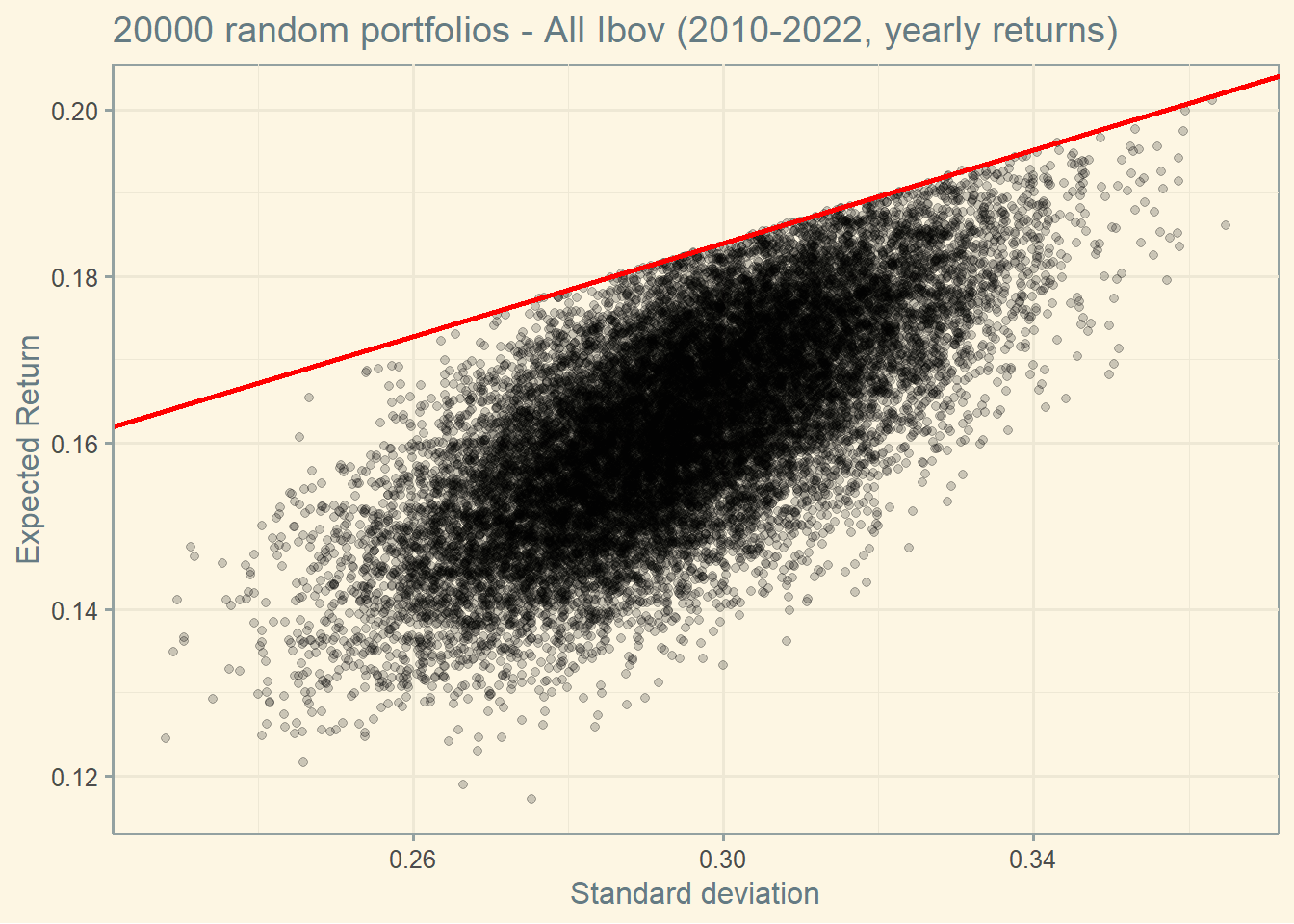
start <-'2010-01-01'end <-'2022-01-01'freq_data <-"yearly"df <-yf_collection_get("IBOV", first_date = start,last_date = end,freq_data = freq_data)stocks <-unique(df$ticker)df <- df %>%select(ref_date)for (i in1:length(stocks)) {data <-yf_get(tickers = stocks[[i]], first_date = start,last_date = end,freq_data = freq_data)data<-data[complete.cases(data),] data<- data %>%select(ref_date, ret_closing_prices)colnames(data) <-c("ref_date", stocks[[i]] )df <-merge(df,data,by="ref_date")}df$ref_date <-NULLcov<-cov(df)ret<-as.vector(colMeans(df))# Random numbers to create the frontierset.seed(100)int <-20000w<-data.frame((replicate(length(stocks),sample(int,rep=TRUE)) / int ))w$sum <-rowSums(w)colnames(w) <-c(stocks, 'Sum')for (i in1:int) {w[i, 1:length(stocks)] <- w[i, 1:length(stocks)] / w[i, ncol(w)]}w$Sum <-NULLw$Sum <-rowSums(w)w$Sum <-NULL# creating final dataframeport <-data.frame(matrix(NA,nrow = int,ncol =2))colnames(port) <-c("Return", "Sd")for (i in1:int) {port[i,1] <-sum( w[i, ] * ret )port[i,2] <-sqrt( as.matrix(w[i, ]) %*%as.matrix(cov) %*%as.matrix(t(w[i, ]) )) }#ggplotggplot(port, aes(x=Sd, y=Return)) +geom_point(alpha=0.2) +theme_solarized() +xlab("Standard deviation") +ylab("Expected Return") +labs(title =paste(int , "random portfolios - All Ibov (2010-2022, Yearly returns)") )
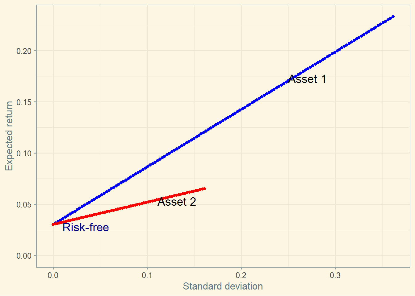
4.5 The Risk-free asset
Let’s include a risk-free asset now to see if anything changes. If this economy is correctly priced, the risk free asset must have an expected return lower than both risky assets. Additionally, the risk-free asset is free of risk, so it will be placed at the y-axis. (Graphs inspired in compfinezbook ).
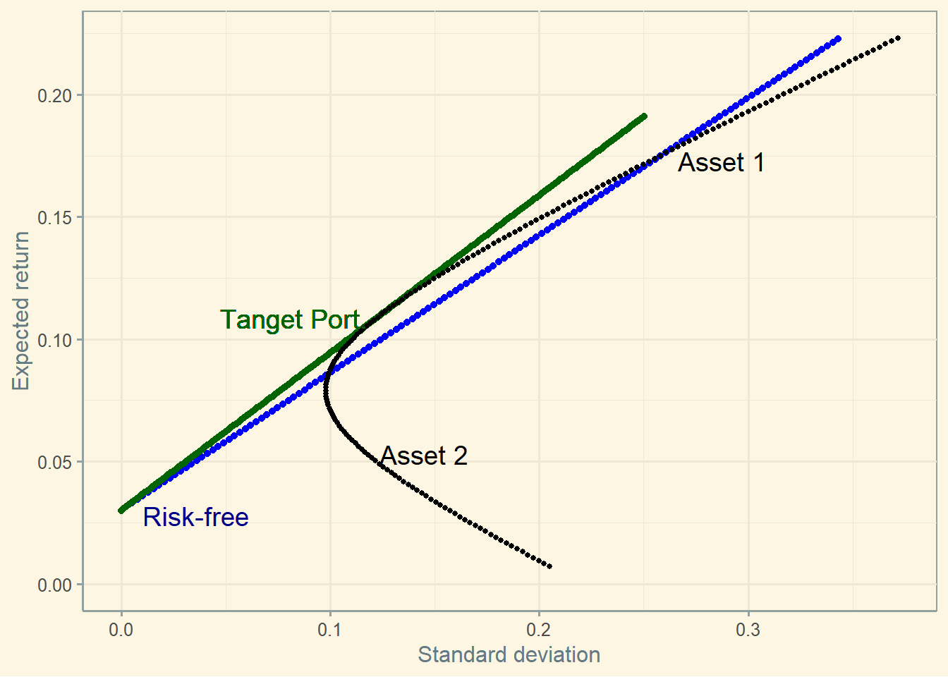
4.5.1 Combining Asset 1 and 2 vs. Asset 1 and risk-free rate
A strategy combining asset 1 and risk-free rate seems to lose comparing to a strategy combining asset 1 and 2.
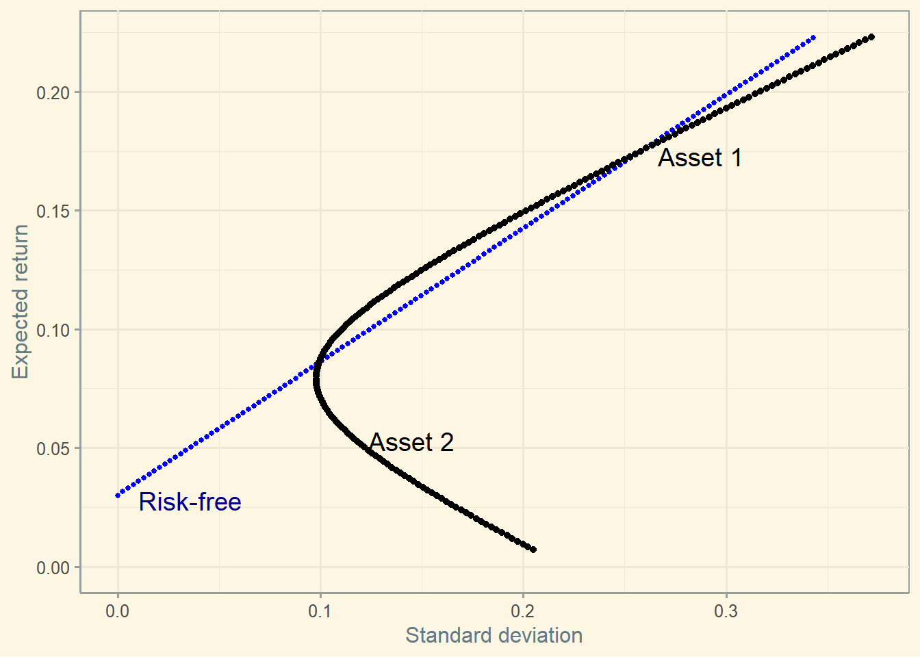
4.5.2 The tangent portfolio
Nevertheless, see what happens if you combine asset 1 and asset 2 and find the tangent portfolio.
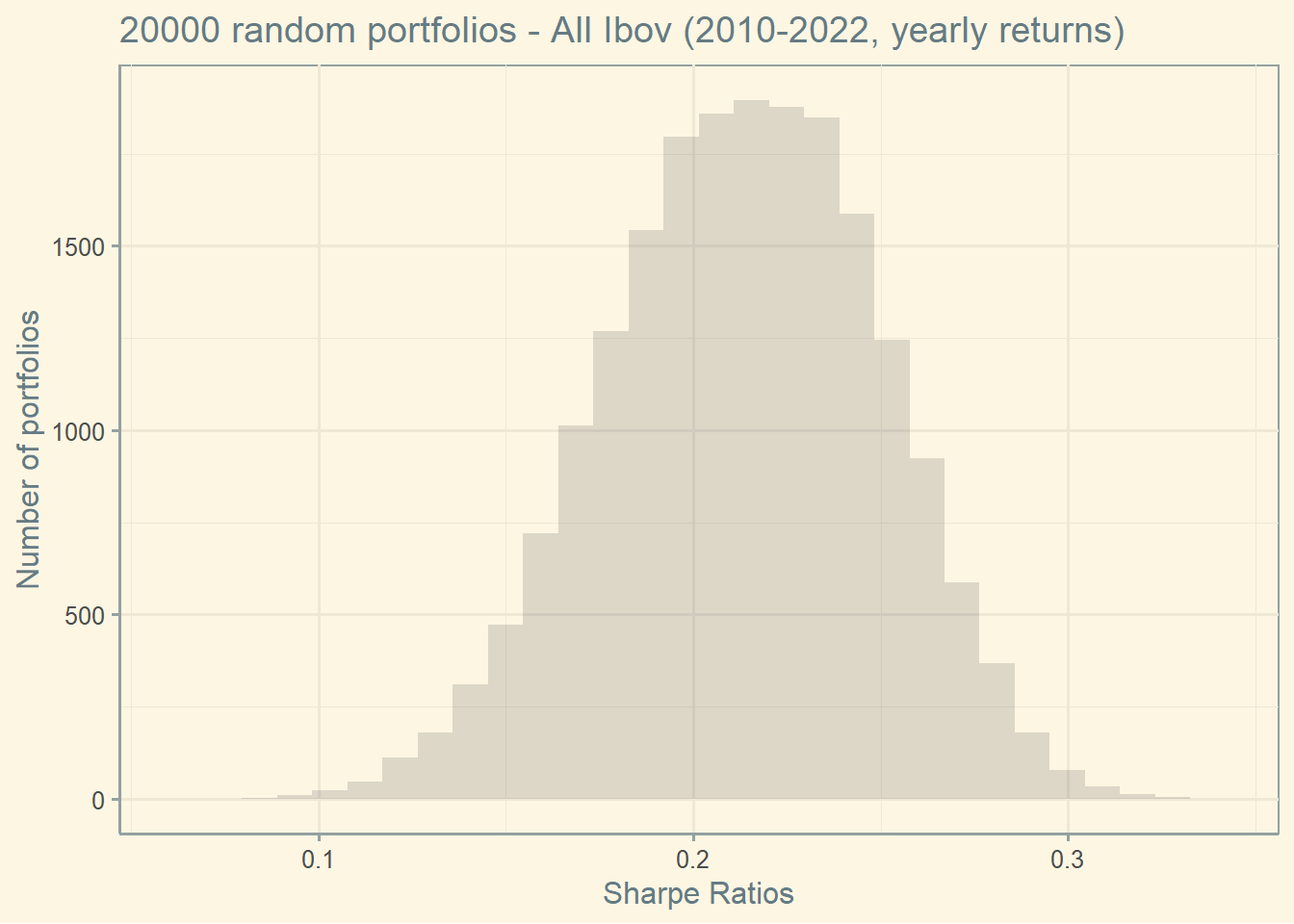
4.6 Sharpe ratio
Let’s see use the same data from the previous graph to create a list of Sharpe ratios. Remember what the Sharpe ratio is:
\[Sharpe\;ratio = \frac{E[R_p]-R_f}{Sd(R_p)}\]
So, for simplicity, I will assume a risk-free rate of 10%, which is low for Brazil these days (but fair in longer windows of time). Also, remember that I using the previous 12 years of data to compute the expected return below for all stocks.
What is a good Sharpe ratio? What is your interpretation about this graph?
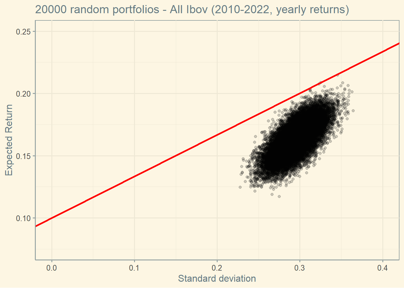
4.7 Capital Market Line (CML)
The slope of the CML is the Sharpe ratio of the efficient portfolio. That is, the highest Sharpe ratio of all portfolios.
This portfolio is called Market portfolio. According to the CAPM, all investors should choose a portfolio on the CML, by holding some combination of the risk-free security and the market portfolio. The CML is represented in red below.
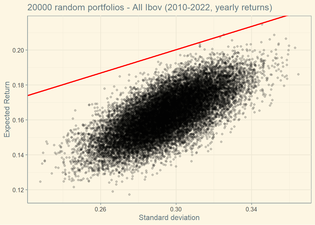
To see the Market portfolio more clearly, I adjusted the axis in the graph below.
Notice that the Market portfolio seems to be an outlier (remember, we are using real data, so outliers are expected to occur).
If we ignore the top 500 Sharpes and assume they are outlier, this is what we get.
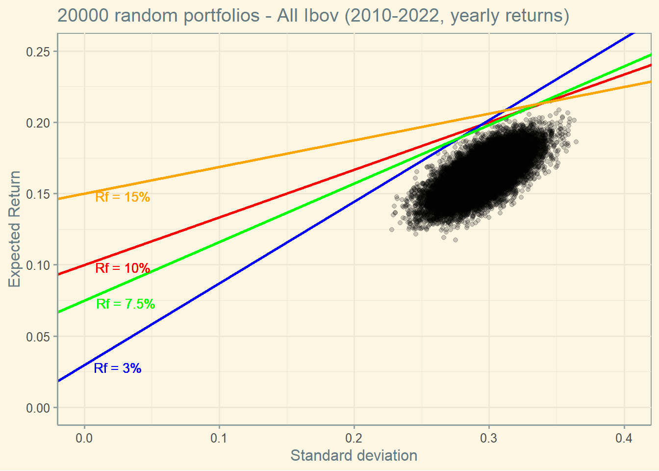
4.7.1 CML with different risk free rates
If the risk free rate changes, all investors are expected to change their allocations.
Notice that the Market portfolio seems to be an outlier (remember, we are using real data, so outliers are expected to occur).
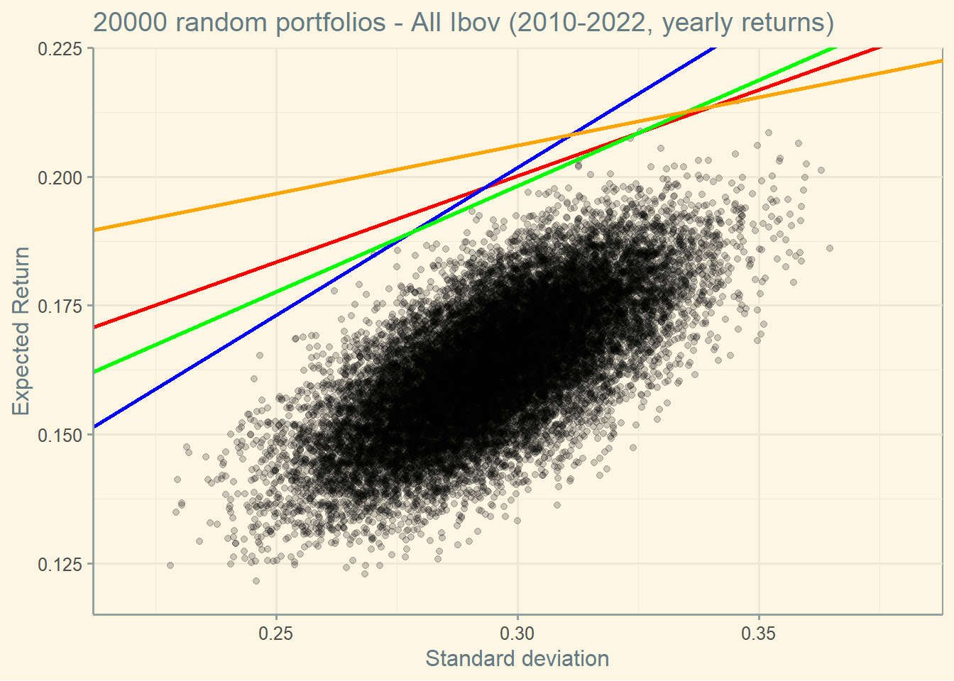
If we zoom in, here is what we find (again, you have to understand the effects of the outliers here and ignore them when making decisions).
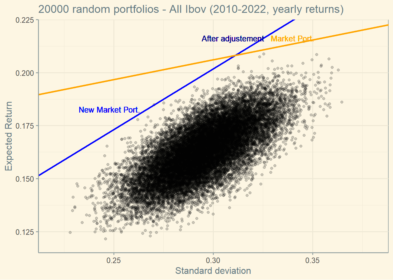
So, here is the interpretation: if the risk free rate drops (let’s say from the orange to the blue line), the market portfolio switches to a safer one (“New Market Port.”).
If investors want the same level of return as before, they will need to adjust their holdings. They will buy the new market portfolio (“New Market Port.”) and will borrow at the risk free rate to get into a levered position (“After adjustment”).
The consequence of all is that, when the risk free rate drops, investor can have the same expected return as before while incurring in much less risk.
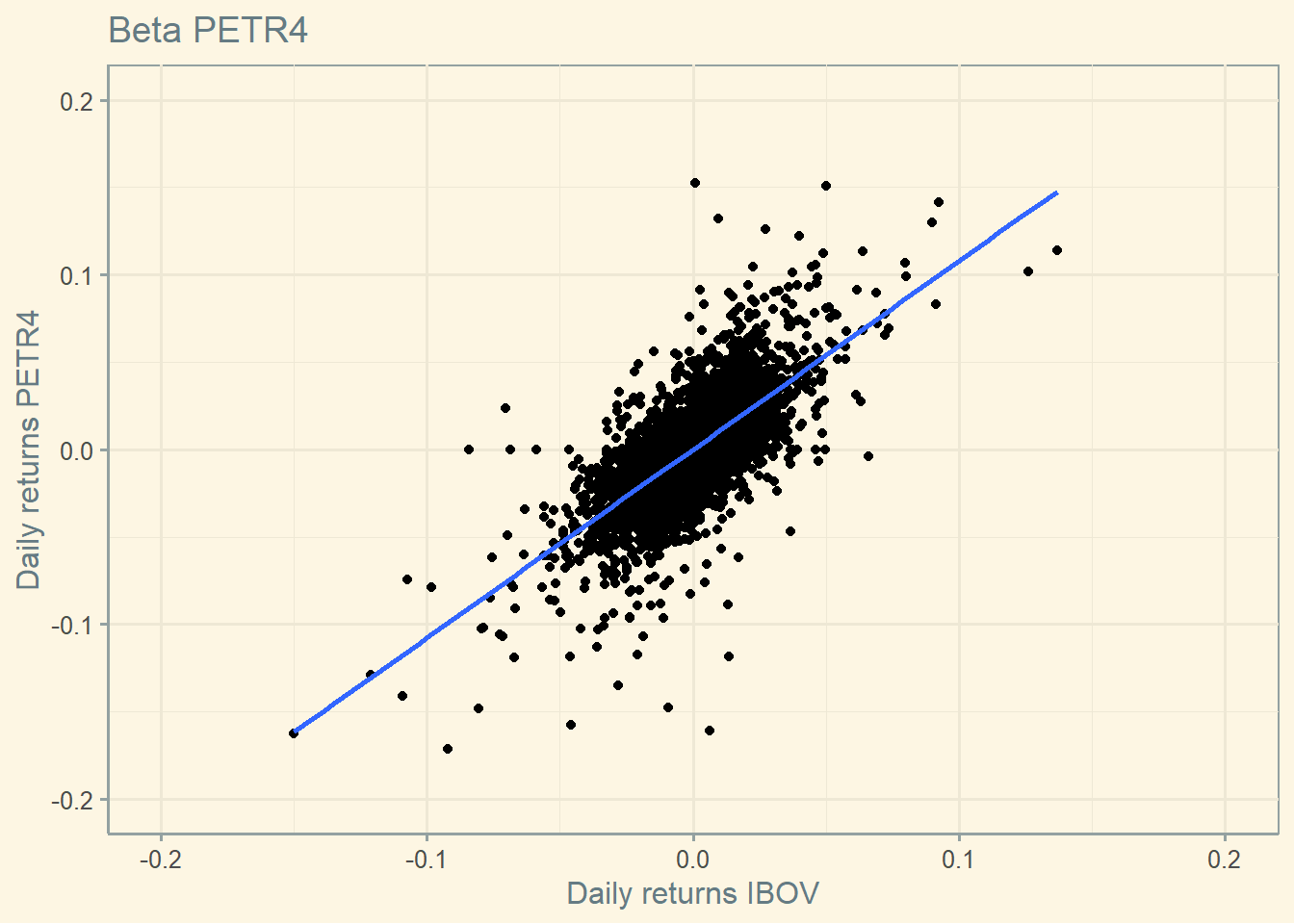
The graph below is a simple plot of the IBOV’s (market) and ABEV’s (a selected stock, see below) returns. We can observe that when the IBOV’s returns are positive, ABEV’s returns are likely positive too. The blue line shows this positive linear relationship. The Beta is the linear coefficient of this line (if you remember the type of function y = a + bx, the linear coefficient is b; this is what we are going to calculate below).
There are two things to understand here: 1) Beta is used in valuation models (such as the CAPM); thus it is essential to calculate it correctly; 2) when Beta is higher than 1, it means the stock is aggressive (meaning that when the market’s return is 1% the stock’s return is higher than 1%). The opposite occurs when the Beta is below 1 (meaning that when the market’s return is 1% the stock’s return is lower than 1%), and the stock is defensive.
The r-squared of the linear regression above represents the proportion of the stock’s total risk that can be explained by the market risk.
##
## Call:
## lm(formula = return.y ~ return.x, data = ret)
##
## Residuals:
##       Min        1Q    Median        3Q       Max
## -0.208393 -0.009931 -0.000161  0.009957  0.151061
##
## Coefficients:
##              Estimate Std. Error t value Pr(>|t|)
## (Intercept) 9.084e-05  2.584e-04   0.352    0.725
## return.x    1.110e+00  1.468e-02  75.611   <2e-16 ***
## ---
## Signif. codes:  0 '***' 0.001 '**' 0.01 '*' 0.05 '.' 0.1 ' ' 1
##
## Residual standard error: 0.01908 on 5455 degrees of freedom
## Multiple R-squared:  0.5117, Adjusted R-squared:  0.5116
## F-statistic:  5717 on 1 and 5455 DF,  p-value: < 2.2e-16
The stock’s beta is 1.11.
The standard error of the beta estimate is: 0.0147.
That is, we can use this error to infer the confidence interval where the “true” beta is.
Additionally, we can say that 51.173 percent of the stock’s risk is explained by market risk.
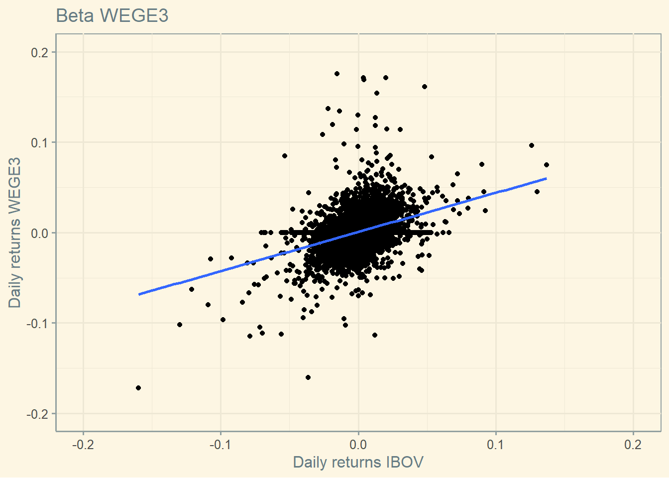
4.8.2 Beta hererogeneity
Notice that different stocks have different betas.
##
## Call:
## lm(formula = return.y ~ return.x, data = ret)
##
## Residuals:
##       Min        1Q    Median        3Q       Max
## -0.164865 -0.008987 -0.000832  0.007810  0.280403
##
## Coefficients:
##              Estimate Std. Error t value Pr(>|t|)
## (Intercept) 0.0008855  0.0002655   3.336 0.000857 ***
## return.x    0.4465415  0.0150793  29.613  < 2e-16 ***
## ---
## Signif. codes:  0 '***' 0.001 '**' 0.01 '*' 0.05 '.' 0.1 ' ' 1
##
## Residual standard error: 0.01961 on 5455 degrees of freedom
## Multiple R-squared:  0.1385, Adjusted R-squared:  0.1383
## F-statistic: 876.9 on 1 and 5455 DF,  p-value: < 2.2e-16
Beta this asset is 0.447.
And around 13.849 percent of this stock’s risk is explained by market risk.
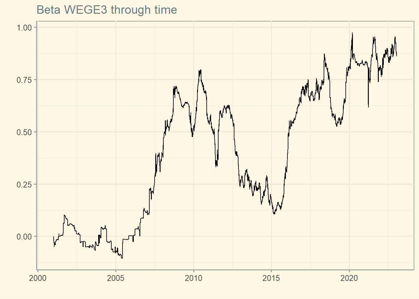
4.8.3 Beta through time
Below we observe that a stock’s beta varies over time (i.e., previous 252 trading days).
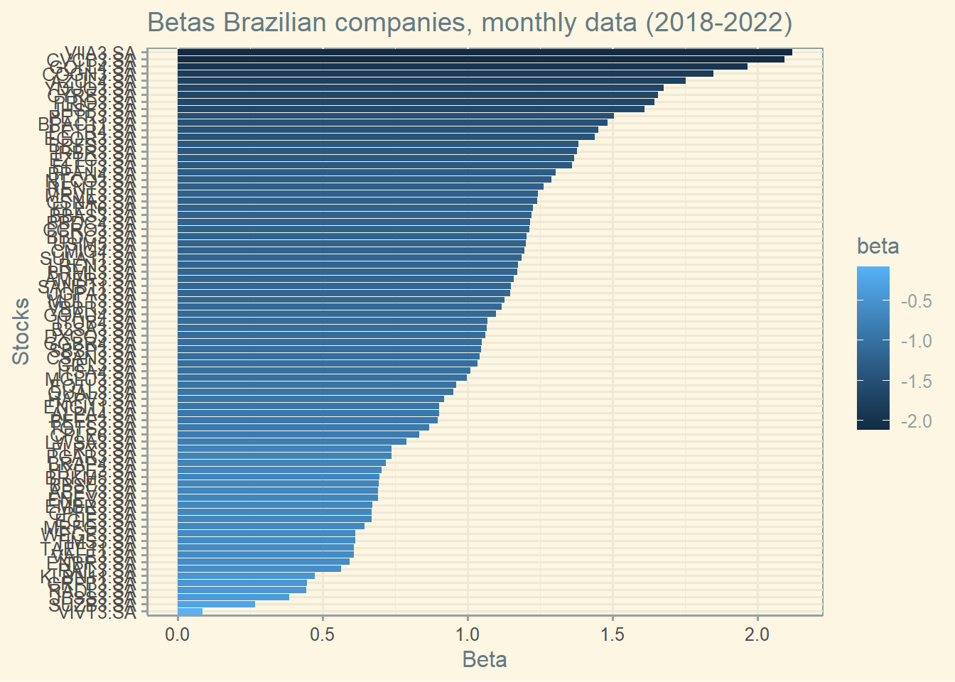
4.8.4 Betas in Brazil
Here is a graph of Betas from Brazilian companies.
start <-'2018-06-01'end <-'2022-06-01'freq_data <-'monthly'ibov <-yf_get(tickers ="^BVSP",first_date = start,last_date = end,thresh_bad_data =0.5,freq_data = freq_data )asset <-yf_collection_get("IBOV", first_date = start,last_date = end,thresh_bad_data =0.5,freq_data = freq_data )ret_ibov <- ibov %>%tq_transmute(select = price_adjusted,mutate_fun = periodReturn,period ='monthly',col_rename ='return')ret_asset <- asset %>%group_by(ticker) %>%tq_transmute(select = price_adjusted,mutate_fun = periodReturn,period ='monthly',col_rename ='return')ret <-left_join(ret_ibov, ret_asset, by =c("ref_date"="ref_date"))var <- ret %>%group_by(ticker) %>%summarise(var =cov(return.x, return.x))cov <- ret %>%group_by(ticker) %>%summarise(cov =cov(return.x, return.y))beta <-merge(cov, var, by ="ticker" )beta$beta <- beta$cov/beta$varggplot(beta, aes(x =reorder(ticker, beta ), y = beta, fill=beta) ) +geom_bar(aes(fill =-beta), position ="dodge", stat="identity")+theme(legend.position="none", axis.text.y =element_blank() )+coord_flip()+labs(y ="Beta", x ="Stocks", title ="Betas Brazilian companies, monthly data (2018-2022)") +theme_solarized()
Here is the list of top and bottom Betas (using monthly data from 2018 until 2022). That is, there is a lot of variation in the betas of Brazilian firms.
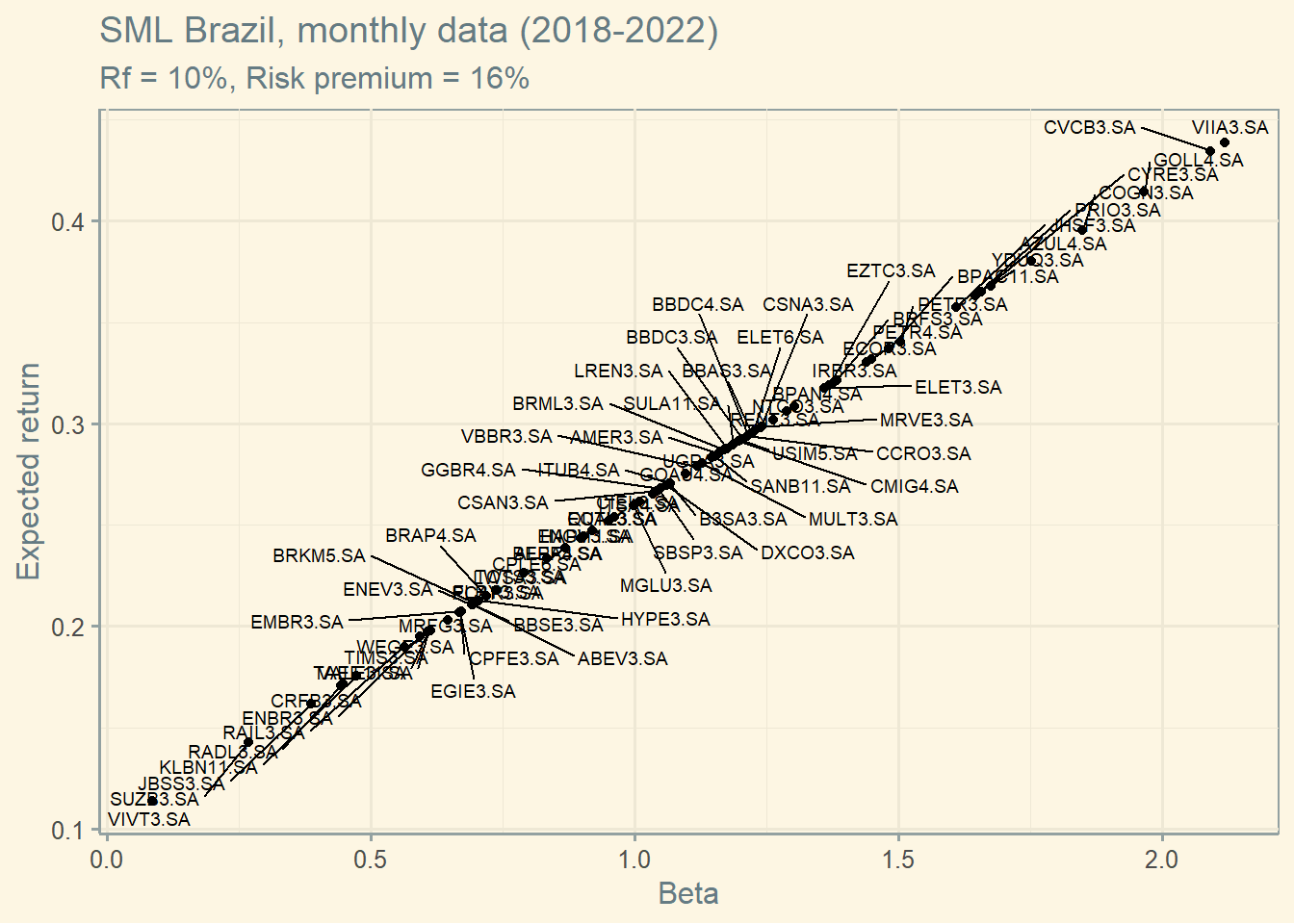
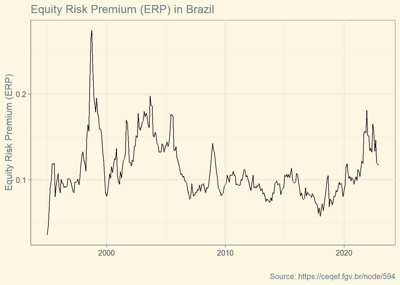
Under the CAPM assumptions, the security market line (SML) is the line along which all individual securities should lie when plotted according to their expected return and beta. To create the graph below, I need estimates to the Brazilian Risk free rate and the Equity Risk Premium. I am using 10% as risk free rate and 16% for the Equity Risk Premium. Equity Risk Premium was based on this website.