2  Macro Brazil

This is a book containing all class notes.

2.1 Selic

#### QUANDL API
# Passos necessC!rios antes de continuar com o cC3digoa baixo
# 1. Acesse https://www.quandl.com/
# 2. Crie uma conta no site
# 3. Obtenha uma API Key
# 4. Adicione sua API Key nos parC"metros abaixo
library(GetQuandlData)
library(ggplot2)
library(ggthemes)
library(GetTDData)

api_KEY <- "Your KEY here"

# Selic BCB/11 or BCB/4390 or BCB/4189 
first_date <- '2000-01-01'
last_date <- '2023-01-01'
selic <- get_Quandl_series(id_in = c('Selic' = 'BCB/4189'),
                               api_key = api_key, 
                               first_date = first_date,
                               last_date = last_date)
cdi <- get_Quandl_series(id_in =  c('CDI' = 'BCB/12'),
                               api_key = api_key, 
                               first_date = first_date,
                               last_date = last_date)
inf <- get_Quandl_series(id_in =  c('Inflation' = 'BCB/433'),
                               api_key = api_key, 
                               first_date = first_date,
                               last_date = last_date)

ggplot(selic, aes( x = ref_date, y= value)) + geom_line() + labs(title = "Selic")+
   theme(axis.text.x = element_text(color = "grey20", size = 15, angle = 0, hjust = .5, vjust = .5, face = "plain"),
        axis.text.y = element_text(color = "grey20", size = 15, angle = 0, hjust = 1, vjust = 0, face = "plain"),  
        axis.title.x = element_text(color = "grey20", size = 15, angle = 0, hjust = .5, vjust = 0, face = "plain"),
        axis.title.y = element_text(color = "grey20", size = 15, angle = 90, hjust = .5, vjust = .5, face = "plain")) +   theme_solarized()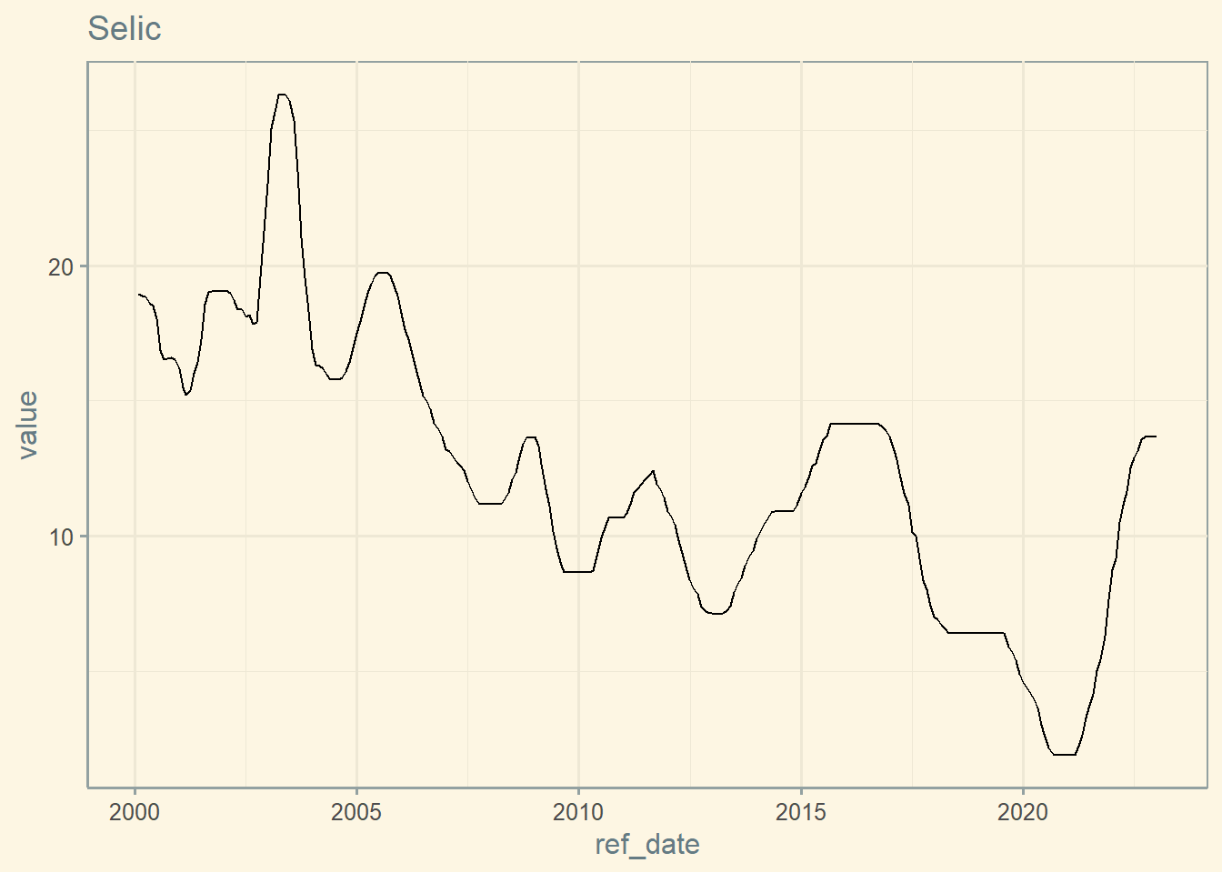

---

2.2 CDI

ggplot(cdi, aes( x = ref_date, y= value)) + geom_line() + labs(title = "CDI")+
   theme(axis.text.x = element_text(color = "grey20", size = 15, angle = 0, hjust = .5, vjust = .5, face = "plain"),
        axis.text.y = element_text(color = "grey20", size = 15, angle = 0, hjust = 1, vjust = 0, face = "plain"),  
        axis.title.x = element_text(color = "grey20", size = 15, angle = 0, hjust = .5, vjust = 0, face = "plain"),
        axis.title.y = element_text(color = "grey20", size = 15, angle = 90, hjust = .5, vjust = .5, face = "plain")) +   theme_solarized()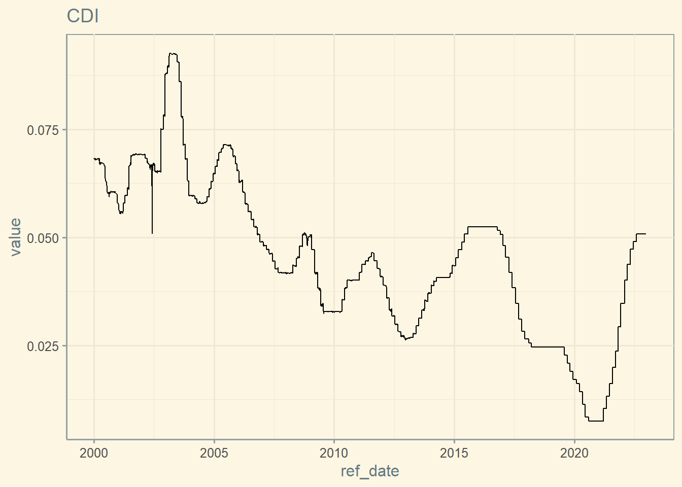

---

2.3 Inflation

ggplot(inf, aes( x = ref_date, y= value)) + geom_line() + labs(title = "Inflation Brazil (IPCA Mensal)")+
   theme(axis.text.x = element_text(color = "grey20", size = 15, angle = 0, hjust = .5, vjust = .5, face = "plain"),
        axis.text.y = element_text(color = "grey20", size = 15, angle = 0, hjust = 1, vjust = 0, face = "plain"),  
        axis.title.x = element_text(color = "grey20", size = 15, angle = 0, hjust = .5, vjust = 0, face = "plain"),
        axis.title.y = element_text(color = "grey20", size = 15, angle = 90, hjust = .5, vjust = .5, face = "plain")) +   theme_solarized()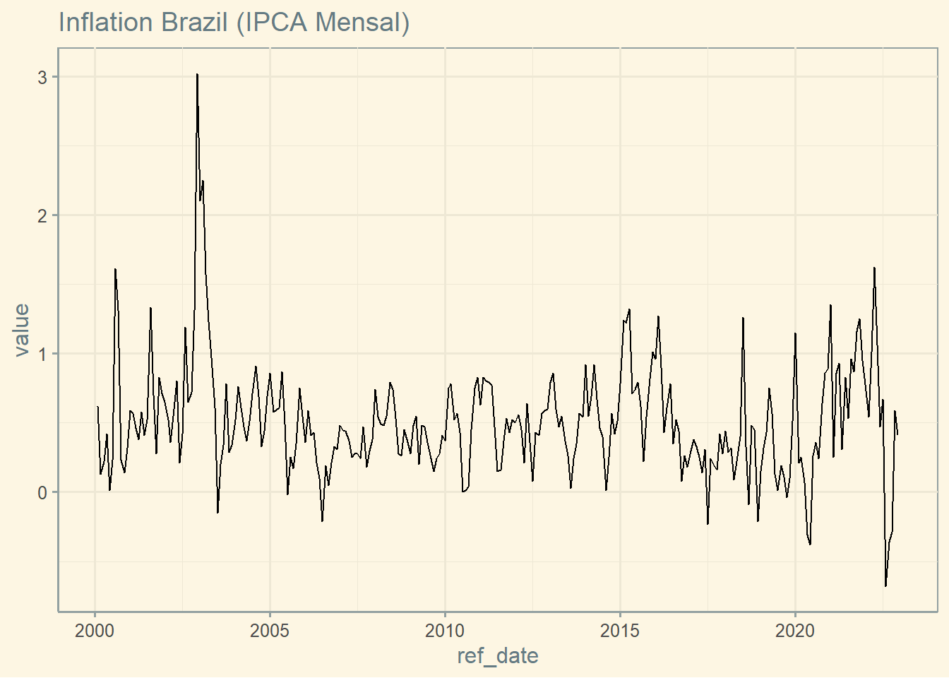

---

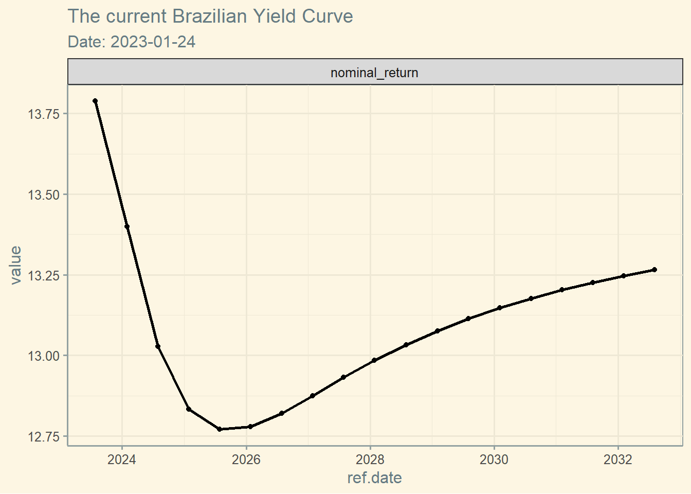
2.4 Term Structure

ettj = get.yield.curve() 
ettj <- subset(ettj, type == "nominal_return" )
ggplot(ettj, aes(x=ref.date, y = value) ) +
        geom_line(size=1) + geom_point() + facet_grid(~type, scales = 'free') + 
        labs(title = paste0('The current Brazilian Yield Curve '),
        subtitle = paste0('Date: ', ettj$current.date[1])) +
   theme(axis.text.x = element_text(color = "grey20", size = 15, angle = 0, hjust = .5, vjust = .5, face = "plain"),
        axis.text.y = element_text(color = "grey20", size = 15, angle = 0, hjust = 1, vjust = 0, face = "plain"),  
        axis.title.x = element_text(color = "grey20", size = 15, angle = 0, hjust = .5, vjust = 0, face = "plain"),
        axis.title.y = element_text(color = "grey20", size = 15, angle = 90, hjust = .5, vjust = .5, face = "plain")) +   theme_solarized()