5  ETFs

This is a book containing all class notes.

5.1 US

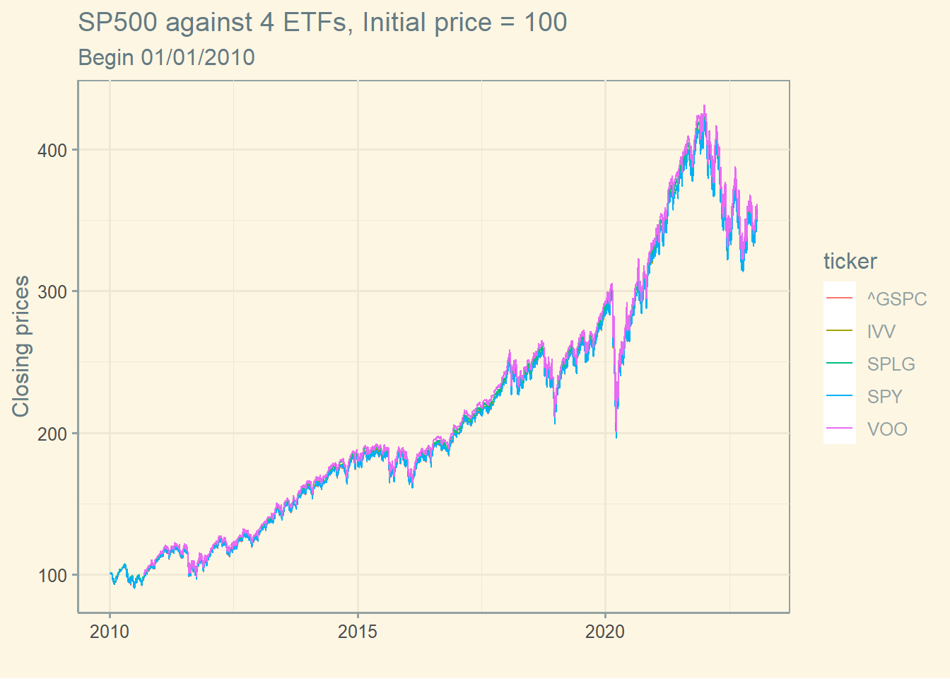
Let’s plot a graph of some Exchange-traded funds (ETFs) available in the US market that follows the SP 500 index. As you can see, the adherence is amazing.

library(yfR)
library(ggplot2)
library(ggthemes)
stocks <-c('SPY', 'IVV','VOO', 'SPLG' , '^GSPC') 
start <-'2010-01-01' 
end   <-Sys.Date()  
data <- yf_get(tickers = stocks, 
                         first_date = start,
                         last_date = end)
data<-data[complete.cases(data),] 
stock1 <- subset(data, ticker == stocks[1])
stock2 <- subset(data, ticker == stocks[2])
stock3 <- subset(data, ticker == stocks[3])
stock4 <- subset(data, ticker == stocks[4])
stock5 <- subset(data, ticker == stocks[5])
stock1$price_close2 <- stock1$price_close  / stock1$price_close[1] * 100
stock2$price_close2 <- stock2$price_close  / stock2$price_close[1] * 100
stock3$price_close2 <- stock3$price_close  / stock3$price_close[1] * 100
stock4$price_close2 <- stock4$price_close  / stock4$price_close[1] * 100
stock5$price_close2 <- stock5$price_close  / stock5$price_close[1] * 100
data2 <- rbind(stock1, stock2, stock3, stock4, stock5)
ggplot(data2, aes(ref_date , price_close2, color=ticker))+
        geom_line() +
        labs(x = "",
             y='Closing prices', 
             title="SP500 against 4 ETFs, Initial price = 100", 
             subtitle = "Begin 01/01/2010") +   theme_solarized()

5.2 Brazil

Here is the same graph for brazilian ETF Bova11. The adherence seems ok.

library(yfR)
library(ggplot2)
library(ggthemes)
stocks <-c('BOVA11.SA', '^BVSP') 
start <-'2010-01-01' 
end   <-Sys.Date()  
data <- yf_get(tickers = stocks, 
                         first_date = start,
                         last_date = end)
data<-data[complete.cases(data),] 
stock1 <- subset(data, ticker == stocks[1])
stock2 <- subset(data, ticker == stocks[2])
stock1$price_close2 <- stock1$price_close  / stock1$price_close[1] * 100
stock2$price_close2 <- stock2$price_close  / stock2$price_close[1] * 100
data2 <- rbind(stock1, stock2)
ggplot(data2, aes(ref_date , price_close2, color=ticker))+
        geom_line() +
        labs(x = "",
             y='Closing prices', 
             title="Ibov against 2 ETFs, Initial price = 100", 
             subtitle = "Begin 01/01/2010") +   theme_solarized()