library(ggplot2)
library(ggthemes)
library(readxl)
library(jtools) # for nice tables of models - https://cran.r-project.org/web/packages/jtools/vignettes/summ.html#summ
data <- read_excel("files/data.xls")7 Real research
7.1 OLS, Panel, Fixed effects, and Random Effects
After uploading the data, tell R the data is panel. You need two identifiers: one for the cross-sectional part (usually, firms in accounting & finance research), and other for the time-series part (usually, year but sometimes can be quarter). The following example uses a panel wit quarterly data.
I am also creating an identifier for industries, which might be useful.
library(dplyr)
data <- data %>% group_by(id )                %>% dplyr::mutate(id_firm = cur_group_id())
data <- data %>% group_by(setor_economatica)  %>% dplyr::mutate(id_ind = cur_group_id())
Now, I am stating to r that I have a dataset in a panel structure.
library(plm)
data <- pdata.frame(data, index=c("id_firm","year"))
Let’s attach the dataset to make things easier.
attach(data)Let’s inspect the dataset. First, let’s see how many observations we have by country:
library('plyr')
count(country)
x freq
1 AR 1497
2 BR 6804
3 CL 3050
4 CO 483
5 MX 2315
6 PE 1928Now, by year.
count(year) x freq
1 1995 624
2 1996 676
3 1997 743
4 1998 749
5 1999 738
6 2000 739
7 2001 681
8 2002 671
9 2003 666
10 2004 687
11 2005 679
12 2006 685
13 2007 739
14 2008 722
15 2009 727
16 2010 717
17 2011 719
18 2012 706
19 2013 701
20 2014 690
21 2015 669
22 2016 663
23 2017 686Now, by industry.
count(setor_economatica) x freq
1 Agro e Pesca 832
2 Alimentos e Beb 1537
3 Comércio 1117
4 Construção 806
5 Eletroeletrônicos 332
6 Energia Elétrica 1539
7 Máquinas Indust 259
8 Mineração 693
9 Minerais não Met 587
10 Outros 2860
11 Papel e Celulose 299
12 Petróleo e Gas 522
13 Química 859
14 Siderur & Metalur 1104
15 Software e Dados 75
16 Telecomunicações 770
17 Textil 845
18 Transporte Serviç 517
19 Veiculos e peças 5247.2 Generating variables
Let’s generate some variables to use later.
data$lev1 <- Debt / (Debt + Equity.market.value)
data$lev2 <- Debt / Total.Assets
data$wc_ta <- wc  / Total.Assets
data$cash_ta <- cash / Total.Assets
data$div_ta <- Dividends / Total.Assets
data$fcf_ta <- Free.cash.flow / Total.Assets
data$tang_ta <- tangible / Total.Assets
data$roa2 <- roa / 100
library(SciViews)
data$size1  <- ln(Total.Assets)
Notice that most variables are ratios and thus are expected to fall in the 0-100% range.
There is one important exception: Size. Size in this example is the natural logarithm of Total Assets (sometimes, studies use the natural logarithm of Total Sales). Taking the natural logarithm is a traditional decision in this type of research.
So, why did I do that in Size but not in the others?
In many cases, you want to use relative differences or percentages change. For instance, GDP growth is usually measured as the growth of each year over the previous year. The same is true for stock prices.
\[GDP\; growth = \frac{GDP_t - GDP_{t-1}}{GDP`{t-1}}\]
This is possible because you always have a previous value to use as base for comparison.
In many cases, you do not have such base for comparison. This is the case of a firm’s Total Assets. What is the natural base for Total Assets? No answer.
Therefore, you take the natural logarithm so that you minimize this concern.
Additionally, keep in mind that the empirical values of Total Assets are often very dissimilar and with huge magnitude. Consider two firms, one with 1 million of total assets, the other with 1 billion. Assume that both firms increased throughout one year their total assets by 1 million. The first firm is twice the size of before, but 1 million make little difference for a billion dollar firm. Taking the logarithm helps you to have a similar base and mitigate the magnitude effect of these changes.
7.3 Summary statistics
library(vtable)
sumtable(data, vars = c('lev1' , 'lev2' , 'wc_ta', 'cash_ta', 'size1' , 'fcf_ta' , 'div_ta', 'roa' , 'tang_ta'))| Variable | N | Mean | Std. Dev. | Min | Pctl. 25 | Pctl. 75 | Max |
|---|---|---|---|---|---|---|---|
| lev1 | 12708 | 0.35 | 0.28 | 0 | 0.11 | 0.55 | 1 |
| lev2 | 12706 | 0.41 | 3.7 | 0 | 0.095 | 0.37 | 244 |
| wc_ta | 15584 | -0.025 | 2.5 | -139 | -0.015 | 0.22 | 1 |
| cash_ta | 15056 | 0.073 | 0.1 | 0 | 0.01 | 0.096 | 1 |
| size1 | 15686 | 20 | 2 | 7.3 | 18 | 21 | 27 |
| fcf_ta | 12426 | 0.091 | 7.4 | -35 | 0.019 | 0.066 | 818 |
| div_ta | 10295 | 0.023 | 1.4 | -0.073 | 0 | 0.0043 | 136 |
| roa | 13689 | 1.6 | 378 | -3656 | -0.47 | 2.4 | 43650 |
| tang_ta | 15600 | 0.4 | 0.25 | 0 | 0.19 | 0.59 | 1.1 |
7.4 Winsorization
Some of the variables have weird values. For instance, the variable \(\frac{Free cash flow}{Total Assets}\) has a maximum value of 817. It means that there is one firm-year observation in which the cash flow of that firm in that year is 817 times the firm’s total assets. This is very odd to say the least.
To avoid this type of problem, we can winsorize our variables.
library(DescTools)
data$w_lev1     <- Winsorize(data$lev1   , probs = c(0.01, 0.99) , na.rm = TRUE)
data$w_lev2     <- Winsorize(data$lev2   , probs = c(0.01, 0.99) , na.rm = TRUE)
data$w_wc_ta    <- Winsorize(data$wc_ta  , probs = c(0.01, 0.99) , na.rm = TRUE)
data$w_cash_ta  <- Winsorize(data$cash_ta, probs = c(0.01, 0.99) , na.rm = TRUE)
data$w_size1    <- Winsorize(data$size1  , probs = c(0.01, 0.99) , na.rm = TRUE)
data$w_fcf_ta   <- Winsorize(data$fcf_ta , probs = c(0.01, 0.99) , na.rm = TRUE)
data$w_div_ta   <- Winsorize(data$div_ta , probs = c(0.01, 0.99) , na.rm = TRUE)
data$w_roa      <- Winsorize(data$roa    , probs = c(0.01, 0.99) , na.rm = TRUE)
data$w_tang_ta  <- Winsorize(data$tang_ta, probs = c(0.01, 0.99) , na.rm = TRUE)
7.5 Panel data
Multiple times are always helpful. That is, in a panel dataset, you have many observations of the same unit in different time periods. This is helpful because you observe the evolution of that unit. Also, this allows to control for time-invariant unobserved heterogeneity at the unit level.
A general representation of a regression using panel data is:
\[Y_{t,i} = \alpha + \beta \times X_{t,i} + \epsilon_{t,i}\]
Notice that each variable has two subscripts, t represents the year = t, and i represents the unit = i. This type of notation is common in empirical research.
7.6 Functional form of relationships
As mentioned before, in many cases, you want to use the logarithm of a variable. This changes the interpretation of the coefficients you estimate.
We have three possible scenarios for regression’s functional forms.
log-log regression: both Y and X are in log values \(ln(Y) = \alpha + \beta \times ln(X) + \epsilon\). The interpretation of \(\beta\) in this case is: \(y\) is \(\beta\) percent higher on average for observations with one percent higher \(x\).
log-level regression: both Y and X are in log values \(ln(Y) = \alpha + \beta \times X + \epsilon\). The interpretation of \(\beta\) in this case is: \(y\) is \(\beta\) percent higher on average for observations with one unit higher \(x\).
level-log regression: both Y and X are in log values \(Y = \alpha + \beta \times ln(X) + \epsilon\). The interpretation of \(\beta\) in this case is: \(y\) is \(\frac{\beta}{100}\) units higher on average for observations with one percent higher \(x\).
Important note: the misspecification of x’s is similar to the omitted variable bias (OVB).
7.7 OLS
This is a plain OLS model using the original data (i.e., not winsorized yet).
ols <- lm(lev1 ~ size1 + fcf_ta + roa + tang_ta + cash_ta + div_ta, data = data)
summary(ols)
Call:
lm(formula = lev1 ~ size1 + fcf_ta + roa + tang_ta + cash_ta +
    div_ta, data = data)

Residuals:
     Min       1Q   Median       3Q      Max
-0.44535 -0.19888 -0.04651  0.16032  1.40432

Coefficients:
             Estimate Std. Error t value Pr(>|t|)
(Intercept) -0.024252   0.031814  -0.762 0.445911
size1        0.018368   0.001564  11.741  < 2e-16 ***
fcf_ta       0.160553   0.105327   1.524 0.127473
roa         -0.001686   0.001054  -1.600 0.109642
tang_ta      0.049239   0.012935   3.807 0.000142 ***
cash_ta     -0.476372   0.031985 -14.893  < 2e-16 ***
div_ta      -1.112794   0.106868 -10.413  < 2e-16 ***
---
Signif. codes:  0 '***' 0.001 '**' 0.01 '*' 0.05 '.' 0.1 ' ' 1

Residual standard error: 0.2462 on 6878 degrees of freedom
  (9192 observations deleted due to missingness)
Multiple R-squared:  0.07463,   Adjusted R-squared:  0.07382
F-statistic: 92.45 on 6 and 6878 DF,  p-value: < 2.2e-16
A nicer looking table.
library(jtools)
export_summs(ols, digits = 3 , model.names = c("OLS") )| OLS | |
|---|---|
| (Intercept) | -0.024 |
| (0.032) | |
| size1 | 0.018 *** |
| (0.002) | |
| fcf_ta | 0.161 |
| (0.105) | |
| roa | -0.002 |
| (0.001) | |
| tang_ta | 0.049 *** |
| (0.013) | |
| cash_ta | -0.476 *** |
| (0.032) | |
| div_ta | -1.113 *** |
| (0.107) | |
| N | 6885 |
| R2 | 0.075 |
| *** p < 0.001; ** p < 0.01; * p < 0.05. | |
Now, we are using the winsorized data.
w_ols <- lm(w_lev1 ~ w_size1 + w_fcf_ta + w_roa + w_tang_ta + w_cash_ta + w_div_ta, data = data)
#summary(w_ols)
export_summs(ols,w_ols ,model.names = c("OLS","OLS (winsorized)"))| OLS | OLS (winsorized) | |
|---|---|---|
| (Intercept) | -0.02 | -0.17 *** |
| (0.03) | (0.03) | |
| size1 | 0.02 *** | |
| (0.00) | ||
| fcf_ta | 0.16 | |
| (0.11) | ||
| roa | -0.00 | |
| (0.00) | ||
| tang_ta | 0.05 *** | |
| (0.01) | ||
| cash_ta | -0.48 *** | |
| (0.03) | ||
| div_ta | -1.11 *** | |
| (0.11) | ||
| w_size1 | 0.03 *** | |
| (0.00) | ||
| w_fcf_ta | -0.03 | |
| (0.11) | ||
| w_roa | -0.01 *** | |
| (0.00) | ||
| w_tang_ta | 0.06 *** | |
| (0.01) | ||
| w_cash_ta | -0.50 *** | |
| (0.03) | ||
| w_div_ta | -3.03 *** | |
| (0.19) | ||
| N | 6885 | 6885 |
| R2 | 0.07 | 0.15 |
| *** p < 0.001; ** p < 0.01; * p < 0.05. | ||
7.8 Heterogeneity across countries
There is a huge literature on capital structure decisions. Let’s see the heterogeneity of leverage across countries. Thus, it makes sense to control for this type of heterogeneity somehow.
library(gplots)
plotmeans(lev1 ~ country, data = data)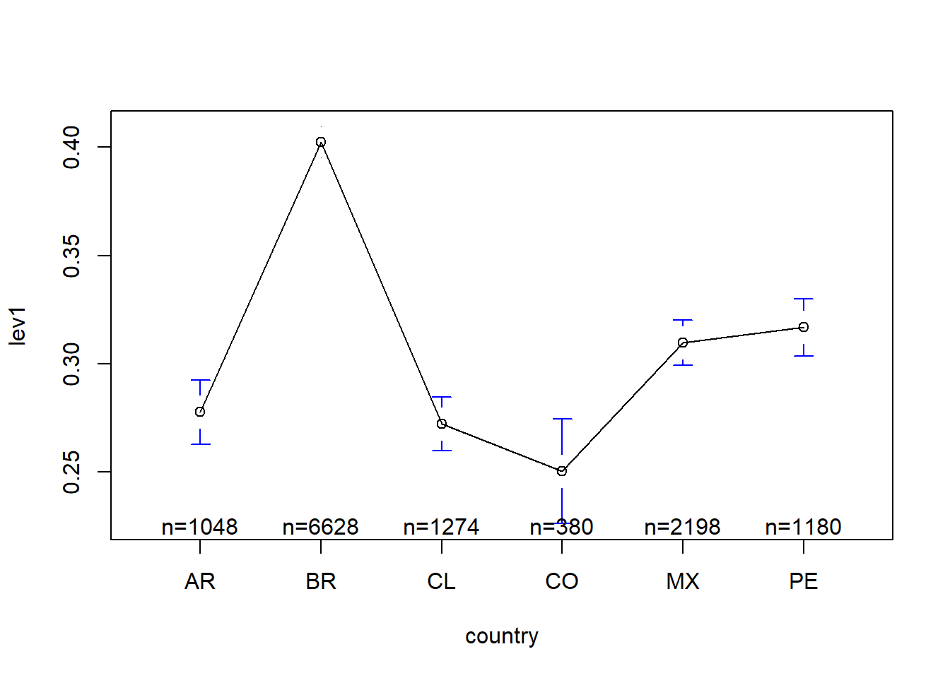
7.9 FE Country
The following example uses fixed effects for countries. Notice that one country is missing.
fe_c <- lm(lev1 ~ size1 + fcf_ta + roa + tang_ta + cash_ta + div_ta  + factor(country) , data = data)
export_summs(fe_c)| Model 1 | |
|---|---|
| (Intercept) | -0.02 |
| (0.03) | |
| size1 | 0.01 *** |
| (0.00) | |
| fcf_ta | 0.11 |
| (0.10) | |
| roa | -0.00 |
| (0.00) | |
| tang_ta | 0.09 *** |
| (0.01) | |
| cash_ta | -0.48 *** |
| (0.03) | |
| div_ta | -1.14 *** |
| (0.11) | |
| factor(country)BR | 0.10 *** |
| (0.01) | |
| factor(country)CL | 0.02 |
| (0.01) | |
| factor(country)CO | 0.11 *** |
| (0.03) | |
| factor(country)MX | 0.03 ** |
| (0.01) | |
| factor(country)PE | 0.09 *** |
| (0.01) | |
| N | 6885 |
| R2 | 0.10 |
| *** p < 0.001; ** p < 0.01; * p < 0.05. | |
Now, we are using fixed effects for countries and years.
fe_cy <- lm(lev1 ~ size1 + fcf_ta + roa + tang_ta + cash_ta + div_ta  + factor(country) + factor(year), data = data)
export_summs(fe_c, fe_cy)| Model 1 | Model 2 | |
|---|---|---|
| (Intercept) | -0.02 | -0.01 |
| (0.03) | (0.04) | |
| size1 | 0.01 *** | 0.02 *** |
| (0.00) | (0.00) | |
| fcf_ta | 0.11 | 0.08 |
| (0.10) | (0.10) | |
| roa | -0.00 | -0.00 |
| (0.00) | (0.00) | |
| tang_ta | 0.09 *** | 0.09 *** |
| (0.01) | (0.01) | |
| cash_ta | -0.48 *** | -0.44 *** |
| (0.03) | (0.03) | |
| div_ta | -1.14 *** | -1.12 *** |
| (0.11) | (0.10) | |
| factor(country)BR | 0.10 *** | 0.10 *** |
| (0.01) | (0.01) | |
| factor(country)CL | 0.02 | 0.01 |
| (0.01) | (0.01) | |
| factor(country)CO | 0.11 *** | 0.08 * |
| (0.03) | (0.03) | |
| factor(country)MX | 0.03 ** | 0.01 |
| (0.01) | (0.01) | |
| factor(country)PE | 0.09 *** | 0.05 ** |
| (0.01) | (0.02) | |
| factor(year)1996 | -0.03 | |
| (0.03) | ||
| factor(year)1997 | -0.08 * | |
| (0.03) | ||
| factor(year)1998 | 0.02 | |
| (0.03) | ||
| factor(year)1999 | -0.03 | |
| (0.03) | ||
| factor(year)2000 | 0.03 | |
| (0.03) | ||
| factor(year)2001 | 0.04 | |
| (0.03) | ||
| factor(year)2002 | 0.04 | |
| (0.03) | ||
| factor(year)2003 | -0.01 | |
| (0.03) | ||
| factor(year)2004 | -0.06 | |
| (0.03) | ||
| factor(year)2005 | -0.08 * | |
| (0.03) | ||
| factor(year)2006 | -0.10 *** | |
| (0.03) | ||
| factor(year)2007 | -0.12 *** | |
| (0.03) | ||
| factor(year)2008 | -0.03 | |
| (0.03) | ||
| factor(year)2009 | -0.12 *** | |
| (0.03) | ||
| factor(year)2010 | -0.13 *** | |
| (0.03) | ||
| factor(year)2011 | -0.08 ** | |
| (0.03) | ||
| factor(year)2012 | -0.07 ** | |
| (0.03) | ||
| factor(year)2013 | -0.06 * | |
| (0.03) | ||
| factor(year)2014 | -0.05 | |
| (0.03) | ||
| factor(year)2015 | 0.00 | |
| (0.03) | ||
| factor(year)2016 | -0.04 | |
| (0.03) | ||
| factor(year)2017 | -0.07 ** | |
| (0.03) | ||
| N | 6885 | 6885 |
| R2 | 0.10 | 0.13 |
| *** p < 0.001; ** p < 0.01; * p < 0.05. | ||
7.10 FE Firms
The most usual regression we estimate in Accounting & Finance is a panel using firms as units. Imagine that you are including one dummy for each firm, just as we included a dummy for each country in the previous example. This is the way to do it.
The strength of a firm fixed effect model is that it controls for time-invariant unobserved heterogeneity at the firm level.
That is, if there is an omitted variable in your model (something that is constant over time that you cannot measure because you do not observe, for instance, the quality of the managerial team), you should use firm fixed effects.
FE is a very traditional and accepted solution in this type of research because our models are always a representation of reality, we can never be sure we are controlling for everything that is important. By including a firm FE you are, at least, safe that you are controlling of omitted variables that do not change over time at the firm level. That is, Firm FE mitigates concerns of omitted variable bias of time-invariant at the firm level.
On top of the firm FE, it is always a good idea to include year FE at the same time, as follows. You do not need to present them in your final paper, but you need to mention them.
fe <- plm(w_lev1 ~ w_size1 + w_fcf_ta + w_roa + w_tang_ta + w_cash_ta + w_div_ta + factor(year) , data = data, model="within")
export_summs(fe, coefs = c("w_size1","w_div_ta","w_fcf_ta","w_roa","w_tang_ta","w_cash_ta"), digits = 3 , model.names = c("FE") )| FE | |
|---|---|
| w_size1 | 0.076 *** |
| (0.004) | |
| w_div_ta | -0.894 *** |
| (0.152) | |
| w_fcf_ta | 0.453 *** |
| (0.117) | |
| w_roa | -0.009 *** |
| (0.001) | |
| w_tang_ta | 0.176 *** |
| (0.019) | |
| w_cash_ta | -0.304 *** |
| (0.029) | |
| nobs | 6885 |
| r.squared | 0.215 |
| adj.r.squared | 0.086 |
| statistic | 57.872 |
| p.value | 0.000 |
| deviance | 108.418 |
| df.residual | 5914.000 |
| nobs.1 | 6885.000 |
| *** p < 0.001; ** p < 0.01; * p < 0.05. | |
More technically (but really not that much), a firm FE model can be represented as follows. That is, you include one fixed term for each firm (again, except for the first firm). Also, I am adding the year FE in the equation below.
\[Y_{t,i} = \beta \times X_{t-1,i} + \alpha_i + \alpha_t+ \epsilon_{t,i}\]
Technically, the inclusion of the FE acts as a transformation of Y and X into differences such as \(y_{t,i} - \bar{y_i}\) and \(x_{t,i} - \bar{x_i}\), where \(\bar{y_i}\) is the mean value of y across all time periods for unit i. As a result, in FE regressions, \(\beta\) shows how much larger y is compared to its mean within the cross-sectional unit. That is, compare two observations of x that are different in terms of their value x compared to the i-specific mean. On average, x is larger that average x by \(\beta\).
Thus, a FE model is a within-unit comparison model and the model is not affected by whether the unit has larger average of X or Y. That is, the estimates are not affected by unobserved confounders that affect either x or y in the same way in all time periods.
Important question: Can you include firm FE and country FE at the same time in a regression? The answer is no. If you try, all the country FE will be dropped due to colinearity with firm FE.
Final notes on FE models:
Notice there is no intercept in the table above. The reason is that the model includes \(i\) intercepts, one for each firm. In some cases, some softwares report an intercept value that is the average of all intercepts. But that is of little value to us.
There are two possible r-squares in FE models: within R-squared and the R-squared (the traditional one). The first is more adequate, because the second uses all intercepts as explanatory variables of y and thus overstates the magnitude of the model’s explanatory power.
7.11 OLS vs FE
At the end of the day, you never can be sure that the FE model is better. So, we can test if it is an improvement over OLS, as follows.
If the p-value low enough then the fixed effects model is the path to go.
pFtest(fe, ols)
    F test for individual effects

data:  w_lev1 ~ w_size1 + w_fcf_ta + w_roa + w_tang_ta + w_cash_ta +  ...
F = 17.45, df1 = 964, df2 = 5914, p-value < 2.2e-16
alternative hypothesis: significant effects
7.12 Random Effects
An alternative to FE models is the RE (random effects) models. In FE models, we assume \(\alpha_i\) is correlated with the other X variables. This makes sense since the unobserved time-invariant characteristics of a firm is expected to be correlated with the observed characteristics of that firm.
If we believe that \(\alpha_i\) is not correlated with X, we should use a RE model. You can estimate as follows.
re <- plm(w_lev1 ~ w_size1 + w_fcf_ta + w_roa + w_tang_ta + w_cash_ta + w_div_ta  , data = data, model="random")
export_summs(fe, re, coefs = c("w_size1","w_div_ta","w_fcf_ta","w_roa","w_tang_ta","w_cash_ta"), digits = 3 , model.names = c("FE", "RE") )| FE | RE | |
|---|---|---|
| w_size1 | 0.076 *** | 0.033 *** |
| (0.004) | (0.003) | |
| w_div_ta | -0.894 *** | -1.336 *** |
| (0.152) | (0.157) | |
| w_fcf_ta | 0.453 *** | 0.307 ** |
| (0.117) | (0.112) | |
| w_roa | -0.009 *** | -0.009 *** |
| (0.001) | (0.001) | |
| w_tang_ta | 0.176 *** | 0.149 *** |
| (0.019) | (0.016) | |
| w_cash_ta | -0.304 *** | -0.410 *** |
| (0.029) | (0.029) | |
| nobs | 6885 | 6885 |
| r.squared | 0.215 | 0.144 |
| adj.r.squared | 0.086 | 0.144 |
| statistic | 57.872 | 856.420 |
| p.value | 0.000 | 0.000 |
| deviance | 108.418 | 146.431 |
| df.residual | 5914.000 | 6878.000 |
| nobs.1 | 6885.000 | 6885.000 |
| *** p < 0.001; ** p < 0.01; * p < 0.05. | ||
7.13 RE vs FE
If you want to test which model is best suited to your dataset, you can test as follows. If the p-value is significant then use FE, if not use RE.
phtest(fe, re)
    Hausman Test

data:  w_lev1 ~ w_size1 + w_fcf_ta + w_roa + w_tang_ta + w_cash_ta +  ...
chisq = 9718.9, df = 6, p-value < 2.2e-16
alternative hypothesis: one model is inconsistent