Let’s learn how to run a regression in R and how to compute the Beta.
First, let’s remember what a linear regression is. In a linear regression, we want to estimate the population paramenters \(\beta_0\) and \(\beta_1\) of the following model.
\[ y = \beta_0 + \beta_1 \times x + \mu\]
In this setting, the variables \(y\) and \(x\) can have several names.
Y
X
Dependent variable
Independent variable
Explained variable
Explanatory variable
Response variable
Control variable
Predicted variable
Predictor variable
Regressand
Regressor
The variable \(\mu\), called the error term, represents all factors that are \(X\) that also affect \(y\). These factors are unobserved in your model. It has specific properties and assumptions.
The parameter \(\beta_0\), i.e., the intercept, is often called the constant term, but it is rarely useful in the type of analysis we’ll run.
We can estimate these parameters as follows:
\[\beta_1 = \frac{Cov(x,y)}{Var(x)}\]
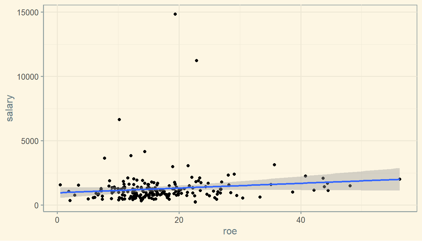
\[\beta_0 = \hat{y} - \hat{\beta_1} \hat{x}\] Let’s estimate Example 2.3 of Wooldridge (2020).
So we see the positive relationship between a firm’s ROE and the Salary paid to the CEO as the regression showed before.
6.3 Regression’s coefficients
Let’s run the regression again.
model <-lm(ceosal1$salary ~ ceosal1$roe)summary(model)## ## Call:## lm(formula = ceosal1$salary ~ ceosal1$roe)## ## Residuals:## Min 1Q Median 3Q Max ## -1160.2 -526.0 -254.0 138.8 13499.9 ## ## Coefficients:## Estimate Std. Error t value Pr(>|t|) ## (Intercept) 963.19 213.24 4.517 1.05e-05 ***## ceosal1$roe 18.50 11.12 1.663 0.0978 . ## ---## Signif. codes: 0 '***' 0.001 '**' 0.01 '*' 0.05 '.' 0.1 ' ' 1## ## Residual standard error: 1367 on 207 degrees of freedom## Multiple R-squared: 0.01319, Adjusted R-squared: 0.008421 ## F-statistic: 2.767 on 1 and 207 DF, p-value: 0.09777
Beta of ROE is 18.501
Standard error of ROE is 11.123.
T-stat of ROE is 1.663.
And p-value is 0.098. So it is barely significantly different from zero at the 10% threshold.
The intercept is 963.191.
The r-squared of the regression is is 963.191.
6.4 Predicting salary
The line from the previous graph contains the estimated salary value of each firm’s CEO.
Let’s say that Firm A shows a ROE of 14.1 and a Salary of 1095. You know that the Beta of the linear regression is 18.501 and the intercept is 963.191. Using these estimates, you can estimate that the salary of Firm A’s CEO is:
\[14.1 \times 18.501 + 963.191 = 1224.058\]
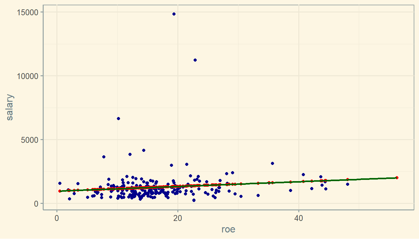
If you do the same to all observations in the dataset, you get the red points below. The darkgreen line connects the points and represents the association between ROE and Salary.
Now, if you can trust your estimates you can estimate (“predict”) the salary for a given new ROE. For instance, you could estimate what is the salary of a new firm that shows a ROE of, let’s say, 30%.
ceosal1$salaryhat <-fitted(model)#summary(ceosal1$salaryhat)ggplot(ceosal1) +geom_point( aes(x=roe, y=salary), color ="darkblue") +geom_point(data=ceosal1, aes(x=roe, y=salaryhat), color ="red") +geom_smooth(data=ceosal1, aes(x=roe, y=salaryhat), color ="darkgreen") +theme_solarized()
6.5 R-squared
We can see in the previous example that the r-squared of the regression is 1.319 percent. This means that the variable ROE explains around 1.3% of the variation of Salary.
Notice in the graph above that there is a distance between the “real” values of salary (i.e., blue points) and the estimated values of salary (i.e., the red points).
This distance is called error or residual.
One thing that you need to understand is that, in a OLS model, the regression line is selected in a way that minimizes the sum of the squared values of the residuals.
You can compute the errors as follows.
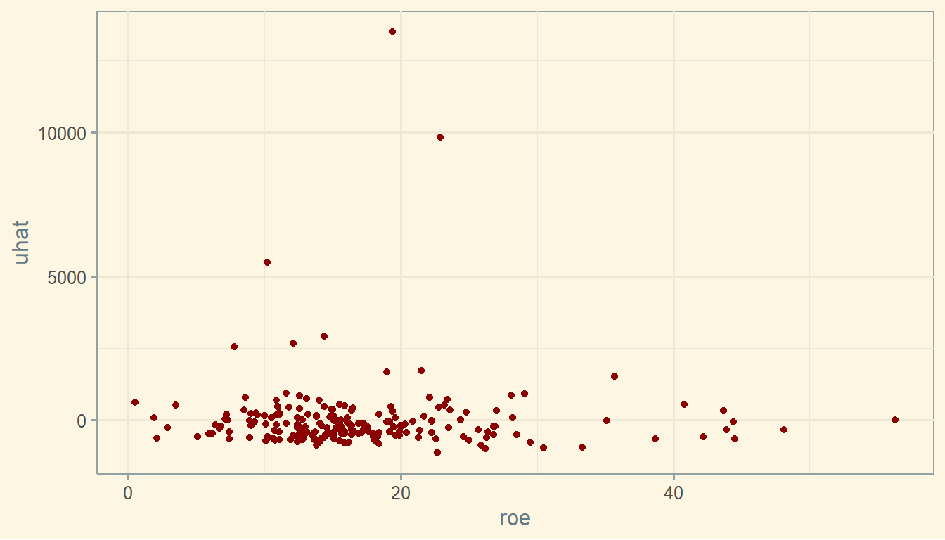
Notice that most residuals are very close to zero. This basically shows that the red points (i.e., the estimated value) are very close to the blue points (i.e., the “real” data) in most of the observations.
But notice there are some observations with large residual, showing they are very far from the estimated value.
ceosal1$uhat <-resid(model)ggplot(ceosal1) +geom_point( aes(x=roe, y=uhat), color ="darkred") +theme_solarized()
The residuals have a mean of zero.
summary(ceosal1$uhat)
##    Min. 1st Qu.  Median    Mean 3rd Qu.    Max.
## -1160.2  -526.0  -254.0     0.0   138.8 13499.9
6.7 Standard error and T-stat
To assess if the variables are significantly related, you need to assess the significance of \(\beta\) coefficients.
Using the example from Wooldridge, we know that the Beta of ROE is 18.501, while the standard error of ROE is 11.123.
The standard error is a measure of the accuracy of your estimate. If you find a large standard error, your estimate does not have good accuracy. Ideally, you would find small standard errors, meaning that your coefficient is accurately estimated. However, you do not have good control over the magnitude of the standard errors.
If you have a large standard error, probably you coefficient will not be significantly different from zero. You can test whether your coefficient is significantly different from zero computing the t-statistics as follows:
If \(t_{\beta}\) is large enough, you can say that \(\beta\) is significantly different from zero. Usually, \(t_{\beta}\) larger than 2 is enough to be significant.
In the previous example, you can find the t-stat manually as follows:
Large t-stats will lead you to low p-values. Usually, we interpret that p-values lower than 10% suggest significance, but you would prefer p-values lower than at least 5%.
You can find the p-values of the previous example as follows.
In this case, p-value is lower than 10% so you can make the case that the relationship is significant at the 10% level. But notice that the relationship is not significant at the level of 5%.
6.8 Confidence intervals
We can further explore significance calculating confidence intervals. First, let’s compute the intervals at 5%. Because our test is a two-tailed test, 5% means 2.5% in each tail.
We can see above that the interval contains the value of Zero (notice that the estimate of ROE goes from a negative to a positive value, thus containing the zero). This means that you cannot separate your estimate of Beta from zero. In other words, your coefficient is not significantly different from zero in this case. This supports the previous finding that the coefficient is not significantly different from zero at the level of 5%.
Let’s see what are the confidence intervals at the level of 10%.
Now, we can see that the interval does not contain zero, which means that Beta is significantly different from zero at the level of 10%. Again, it confirms the previous findings.