5  Selection problem

Imagine that the population contains 5000 units, from which you can observe only 50.

You want to run a linear model to understand the relationship between x and Y.

The “true” beta of this relationship is as follows. By “true” I mean the beta you would get should you observe the population (remember though that you don’t).

summary(lm(df$y ~ df$x))
## 
## Call:
## lm(formula = df$y ~ df$x)
## 
## Residuals:
##      Min       1Q   Median       3Q      Max 
## -2527.44 -1230.21     4.28  1246.20  2510.94 
## 
## Coefficients:
##              Estimate Std. Error t value Pr(>|t|)    
## (Intercept) 2.549e+03  4.103e+01   62.13   <2e-16 ***
## df$x        1.871e-01  1.407e-02   13.30   <2e-16 ***
## ---
## Signif. codes:  0 '***' 0.001 '**' 0.01 '*' 0.05 '.' 0.1 ' ' 1
## 
## Residual standard error: 1435 on 4998 degrees of freedom
## Multiple R-squared:  0.03416,    Adjusted R-squared:  0.03397 
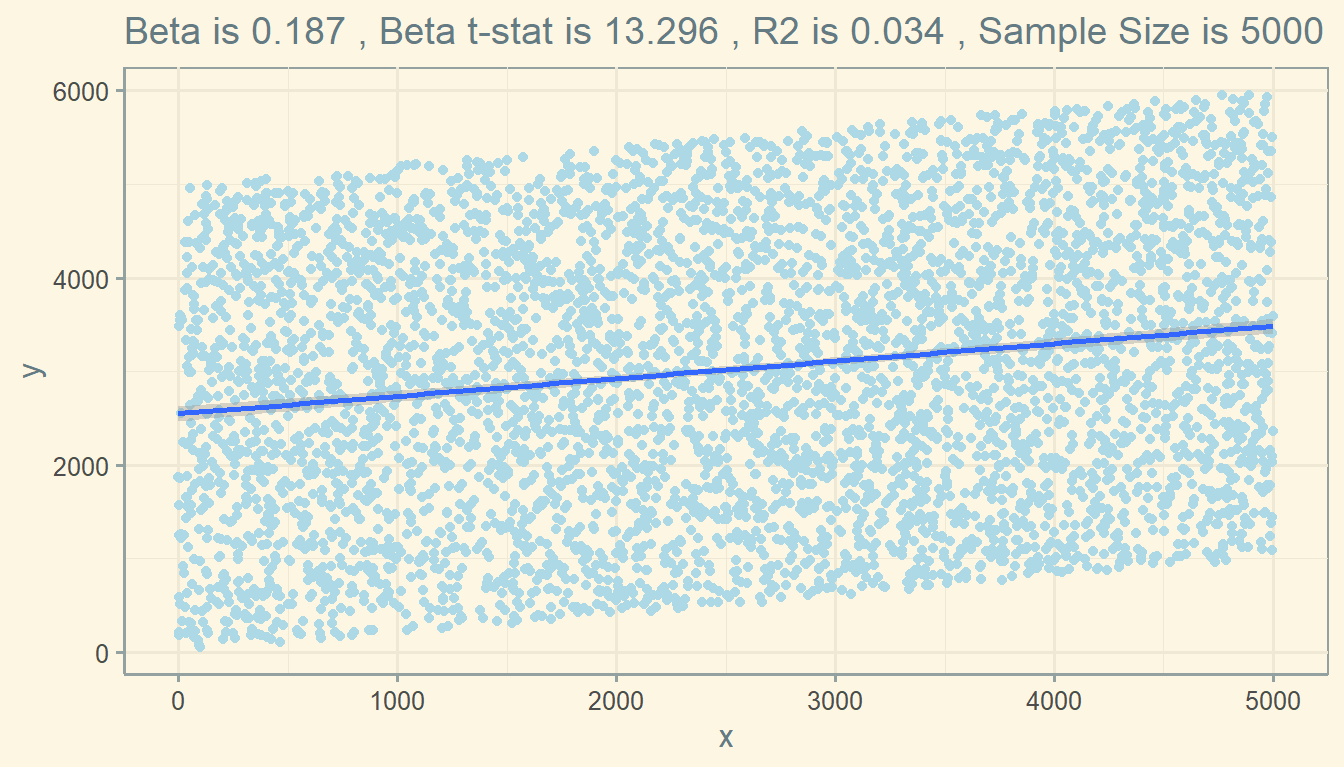
## F-statistic: 176.8 on 1 and 4998 DF,  p-value: < 2.2e-16

So the “true” beta is 0.187. And the t-stat is 13.296

Plotting this relationship in a graph, you get:

---

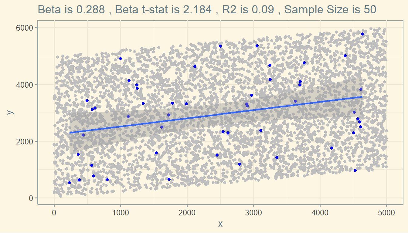
If you run a linear model using the sample you can observe, you might get this.

---

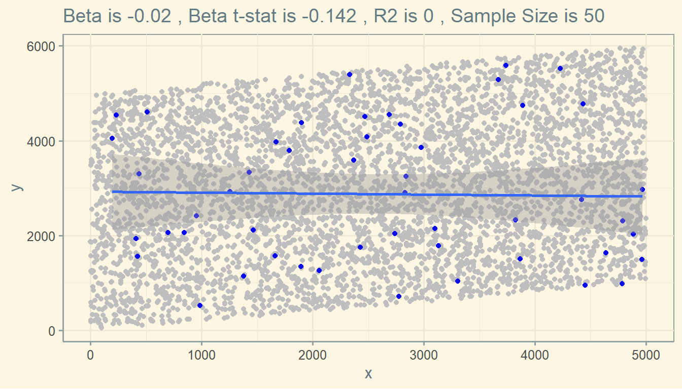
Or maybe this:

---

Or maybe this:

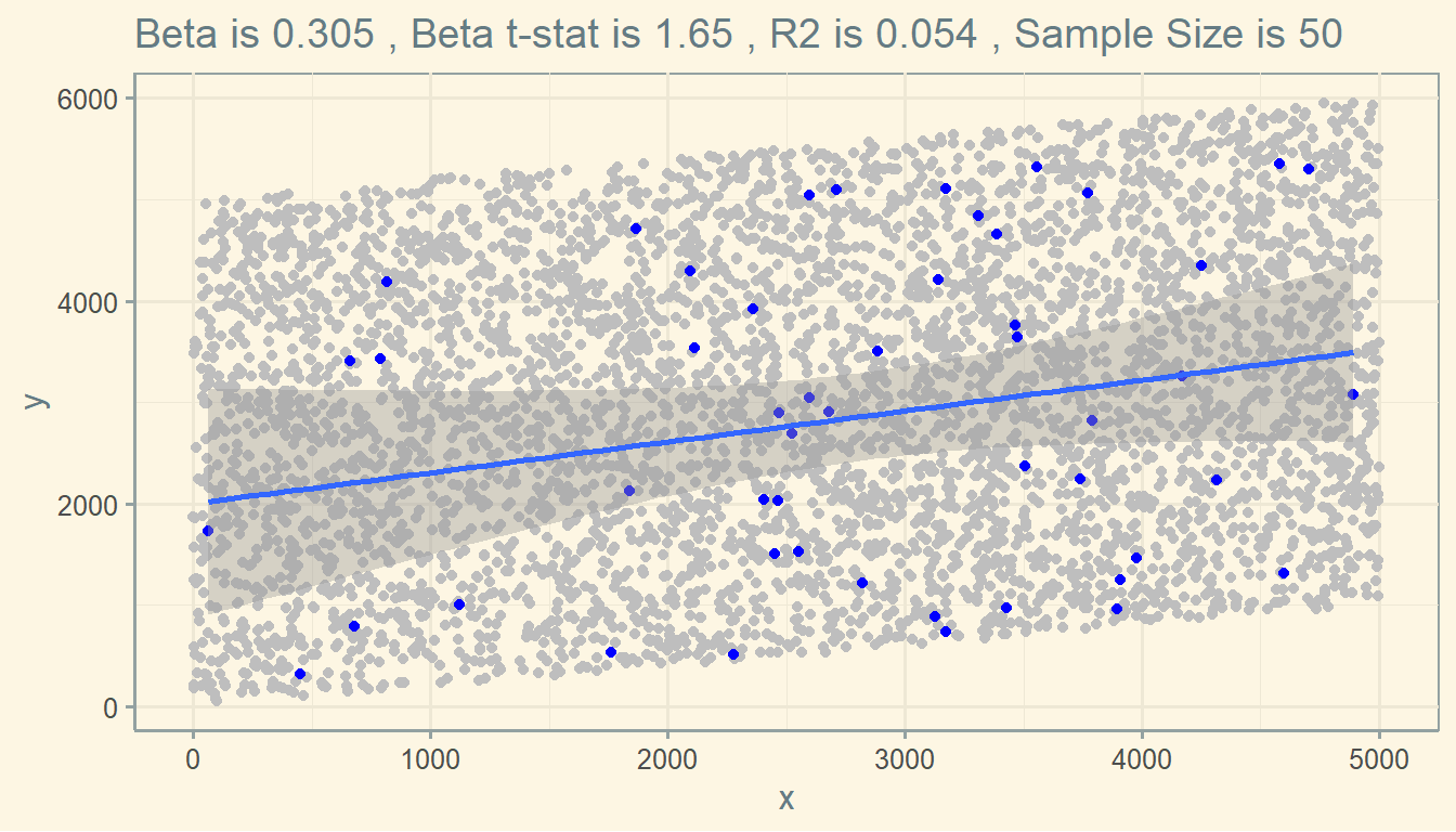
Or maybe several other estimates.

So, the takeaway is: always remember that you can only observe a sample of the population. If the sample you observe is biased, you will get biased estimates.